mixedmath

In my previous note, I described some of the main ideas behind the paper "When are there continuous choices for the mean value abscissa?" that I wrote joint with Miles Wheeler. In this note, I discuss the process behind generating the functions and figures in our paper.

Our functions came in two steps: we first need to choose which functions to plot; then we need to figure out how to graphically solve their general mean value abscissae problem.

Afterwards, we can decide how to plot these functions well.

Choosing the right functions to plot

The first goal is to find the right functions to plot. From the discussion in our paper, this amounts to specifying certain local conditions of the function. And for a first pass, we only used these prescribed local conditions.

The idea is this: to study solutions to the mean value problem, we look at the zeroes of the function $$ F(b, c) = \frac{f(b) - f(a)}{b - a} - f'(c). $$ When $F(b, c) = 0$, we see that $c$ is a mean value abscissa for $f$ on the interval $(a, b)$.

By the implicit function theorem, we can solve for $c$ as a function of $b$ around a given solution $(b_0, c_0)$ if $F_c(b_0, c_0) \neq 0$. For this particular function, $F_c(b_0, c_0) = -f''(c_0)$.

More generally, it turns out that the order of vanishing of $f'$ at $b_0$ and $c_0$ governs the local behaviour of solutions in a neighborhood of $(b_0, c_0)$.

To make figures, we thus need to make functions with prescribed orders of vanishing of $f'$ at points $b_0$ and $c_0$, where $c_0$ is itself a mean value abscissa for the interval $(a_0, b_0)$.

Without loss of generality, it suffices to consider the case when $f(a_0) = f(b_0) = 0$, as otherwise we can study the function $$ g(x) = f(x) - \left( \frac{f(b_0) - f(a_0)}{b_0 - a_0}(x - a_0) + f(a_0) \right), $$ which has $g(a_0) = g(b_0) = 0$, and those triples $(a, b, c)$ which solve this for $f$ also solve this for $g$.

And for consistency, we made the arbitrary decisions to have $a_0 = 0$, $b_0 = 3$, and $c_0 = 1$. This decision simplified many of the plotting decisions, as the important points were always $0$, $1$, and $3$.

A first idea

Thus the first task is to be able to generate functions $f$ such that:

1. $f(0) = 0$,
2. $f(3) = 0$,
3. $f'(1) = 0$ (so that $1$ is a mean value abscissa), and
4. $f'(x)$ has prescribed order of vanishing at $1$, and
5. $f'(x)$ has prescribed order of vanishing at $3$.

These conditions can all be met by an appropriate interpolating polynomial. As we are setting conditions on both $f$ and its derivatives at multiple points, this amounts to the fundamental problem in Hermite interpolation. Alternatively, this amounts to using Taylor's theorem at multiple points and then using the Chinese Remainder Theorem over $\mathbb{Z}[x]$ to combine these polynomials together.

There are clever ways of solving this, but this task is so small that it doesn't require cleverness. In fact, this is one of the laziest solutions we could think of. We know that given $n$ Hermite conditions, there is a unique polynomial of degree $n - 1$ that interpolates these conditions. Thus we

1. determine the degree of the polynomial,
2. create a degree $n-1$ polynomial with variable coefficients in sympy,
3. have sympy symbolically compute the relations the coefficients must satisfy,
4. ask sympy to solve this symbolic system of equations.

In code, this looks like

import sympy
from sympy.abc import X, B, C, D    # Establish our variable names
def interpolate(conds):
    """
    Finds the polynomial of minimal degree that solves the given Hermite conditions.

    conds is a list of the form
      [(x1, r1, v1), (x2, r2, v2), ...]
    where the polynomial p is to satisfy p^(r_1) (x_1) = v_1, and so on.
    """
    # the degree will be one less than the number of conditions
    n = len(conds)

    # generate a symbol for each coefficient
    A = [sympy.Symbol("a[%d]" % i) for i in range(n)]

    # generate the desired polynomial symbolically
    P = sum([A[i] * X**i for i in range(n)])

    # generate the equations the polynomial must satisfy
    #
    # for each (x, r, v), sympy evaluates the rth derivative of P wrt X,
    # substitutes x in for X, and requires that this equals v.
    EQNS = [sympy.diff(P, X, r).subs(X, x) - v for x, r, v in conds]

    # solve this system for the coefficients A[n]
    SOLN = sympy.solve(EQNS, A)

    return P.subs(SOLN)

We note that we use the convention that a sympy symbol for something is capitalized. For example, we think of the polynomial as being represented by $$ p(x) = a(0) + a(1)x + a(2)x^2 + \cdots + a(n)x^n. $$ In sympy variables, we think of this as

P = A[0] + A[1] * X + A[2] * X**2 + ... + A[n] * X**n

With this code, we can ask for the unique degree 1 polynomial which is $1$ at $1$, and whose first derivative is $2$ at $1$.

> interpolate([(1, 0, 1), (1, 1, 2)])
2*X - 1

Indeed, $2x - 1$ is this polynomial.

Too rigid

We have now produced a minimal Hermite solver. But there is a major downside: the unique polynomial exhibiting the necessary behaviours we required is essentially never a good didactic example. We don't just want plots — we want beautiful, simple plots.

Add knobs to turn

We add two conditions for additional control, and hopefully for additional simplicity of the resulting plot.

Firstly, we added the additional constraint that $f(1) = 1$. This is small, but it's a small prescribed value. So now at least all three points of interest will fit within a $[0, 3] \times [0, 3]$ box.

Secondly, we also allow the choice of the value of the first nonvanishing derivatives at $1$ and $3$. In reality, we treat these as parameters to change the shape of the resulting graph. Roughly speaking, if the order of vanishing of $f(x) - f(1)$ is $k$ at $1$, then near $1$ the approximation $f(x) \approx f^{(k)}(1) x^k/k!$ is true. Morally, the larger the value of the derivative, the more the graph will resemble $x^k$ near that point.

In code, we implemented this by making functions that will add the necessary Hermite conditions to our input to interpolate.

# We fix the values of a0, b0, c0.
a0 = 0
b0 = 3
c0 = 1

# We require p(a0) = 0, p(b0) = 0, p(c0) = 1, p'(c0) = 0.
BASIC_CONDS = [(a0, 0, 0), (b0, 0, 0), (c0, 0, 1), (c0, 1, 0)]

def c_degen(n, residue):
    """
    Give Hermite conditions for order of vanishing at c0 equal to `n`, with
    first nonzero residue `residue`.

    NOTE: the order `n` is in terms of f', not of f. That is, this is the amount
    of additional degeneracy to add.  This may be a source of off-by-one errors.
    """
    return [(c0, 1 + i, 0) for i in range(1, n + 1)] + [(c0, n + 2, residue)]


def b_degen(n, residue):
    """
    Give Hermite conditions for order of vanishing at b0 equal to `n`, with
    first nonzero residue `residue`.
    """
    return [(b0, i, 0) for i in range(1, n + 1)] + [(b0, n + 1, residue)]

def poly_with_degens(nc=0, nb=0, residue_c=3, residue_b=3):
    """
    Give unique polynomial with given degeneracies for this MVT problem.

    `nc` is the order of vanishing of f' at c0, with first nonzero residue `residue_c`.
    `nb` is the order of vanishing of f at b0, with first nonzero residue `residue_b`.
    """
    conds = BASIC_CONDS + c_degen(nc, residue_c) + b_degen(nb, residue_b)
    return interpolate(conds)

Then apparently the unique polynomial degree $5$ polynomial $f$ with $f(0) = f(3) = f'(1) = 0$, $f(1) = 1$, and $f''(1) = f'(3) = 3$ is given by

> poly_with_degens()
11*X**5/16 - 21*X**4/4 + 113*X**3/8 - 65*X**2/4 + 123*X/16

Too many knobs

In principle, this is a great solution. And if you turn the knobs enough, you can get a really nice picture. But the problem with this system (and with many polynomial interpolation problems) is that when you add conditions, you can introduce many jagged peaks and sudden changes. These can behave somewhat unpredictably and chaotically — small changes in Hermite conditions can lead to drastic changes in resulting polynomial shape.

What we really want is for the interpolator to give a polynomial that doesn't have sudden changes.

Minimize change

The problem: the polynomial can have really rapid changes that makes the plots look bad.

The solution: minimize the polynomial's change.

That is, if $f$ is our polynomial, then its rate of change at $x$ is $f'(x)$. Our idea is to "minimize" the average size of the derivative $f'$ — this should help keep the function in frame. There are many ways to do this, but we want to choose one that fits into our scheme (so that it requires as little additional work as possible) but which works well.

We decide that we want to focus our graphs on the interval $(0, 4)$. Then we can measure the average size of the derivative $f'$ by its L2 norm on $(0, 4)$: $$ L2(f) = \int_0^4 (f'(x))^2 dx. $$

We add an additional Hermite condition of the form (pt, order, VAL) and think of VAL as an unknown symbol. We arbitrarily decided to start with $pt = 2$ (so that now behavior at the points $0, 1, 2, 3$ are all being controlled in some way) and $order = 1$. The point itself doesn't matter very much, since we're going to minimize over the family of polynomials that interpolate the other Hermite conditions with one degree of freedom.

In other words, we are adding in the condition that $f'(2) = VAL$ for an unknown VAL.

We will have sympy compute the interpolating polynomial through its normal set of (explicit) conditions as well as the symbolic condition (2, 1, VAL). Then $f = f(\mathrm{VAL}; x)$.

Then we have sympy compute the (symbolic) L2 norm of the derivative of this polynomial with respect to VAL over the interval $(0, 4)$, $$L2(\mathrm{VAL}) = \int_0^x f'(\mathrm{VAL}; x)^2 dx.$$

Finally, to minize the L2 norm, we have sympy compute the derivative of $L2(\mathrm{VAL})$ with respect to VAL and find the critical points, when the derivative is equal to $0$. We choose the first one to give our value of VAL.^{1 1}In principle, I suppose we could be finding a local maximum. We could guarantee that we're finding the minimum by choosing the critical point that minimized the L2 norm. Choosing val very large in magnitude makes the L2 norm very large, and so the minimum will be one of the critical points.

In code, this looks like

def smoother_interpolate(conds, ctrl_point=2, order=1, interval=(0,4)):
    """
    Find the polynomial of minimal degree that interpolates the Hermite
    conditions in `conds`, and whose behavior at `ctrl_point` minimizes the L2
    norm on `interval` of its derivative.
    """
    # Add the symbolic point to the conditions.
    # Recall that D is a sympy variable
    new_conds = conds + [(ctrl_point, order, D)]

    # Find the polynomial interpolating `new_conds`, symbolic in X *and* D
    P = interpolate(new_conds)

    # Compute L2 norm of the derivative on `interval`
    L2 = sympy.integrate(sympy.diff(P, X)**2, (X, *interval))

    # Take the first critical point of the L2 norm with respect to D
    SOLN = sympy.solve(sympy.diff(L2, D), D)[0]

    # Substitute the minimizing solution in for D and return
    return P.subs(D, SOLN)


def smoother_poly_with_degens(nc=0, nb=0, residue_c=3, residue_b=3):
    """
    Give unique polynomial with given degeneracies for this MVT problem whose
    derivative on (0, 4) has minimal L2 norm.

    `nc` is the order of vanishing of f' at c0, with first nonzero residue `residue_c`.
    `nb` is the order of vanishing of f at b0, with first nonzero residue `residue_b`.

    """
    conds = BASIC_CONDS + c_degen(nc, residue_c) + b_degen(nb, residue_b)
    return smoother_interpolate(conds)

Then apparently the polynomial degree $6$ polynomial $f$ with $f(0) = f(3) = f'(1) = 0$, $f(1) = 1$, and $f''(1) = f'(3) = 3$, and with minimal L2 derivative norm on $(0, 4)$ is given by

> smoother_poly_with_degens()
-9660585*X**6/33224848 + 27446837*X**5/8306212 - 232124001*X**4/16612424
  + 57105493*X**3/2076553 - 858703085*X**2/33224848 + 85590321*X/8306212

> sympy.N(smoother_poly_with_degens())
-0.290763858423069*X**6 + 3.30437472580762*X**5 - 13.9729157526921*X**4
  + 27.5001374874612*X**3 - 25.8452073279613*X**2 + 10.3043747258076*X

Is it much better? Let's compute the L2 norms.

> interval = (0, 4)
> sympy.N(sympy.integrate(sympy.diff(poly_with_degens(), X)**2, (X, *interval)))
1865.15411706349

> sympy.N(sympy.integrate(sympy.diff(smoother_poly_with_degens(), X)**2, (X, *interval)))
41.1612799050325

That's beautiful. And you know what's better? Sympy did all the hard work.

For comparison, we can produce a basic plot using numpy and matplotlib.

import matplotlib.pyplot as plt
import numpy as np

def basic_plot(F, n=300):
    fig = plt.figure(figsize=(6, 2.5))
    ax = fig.add_subplot(1, 1, 1)
    b1d = np.linspace(-.5, 4.5, n)
    f = sympy.lambdify(X, F)(b1d)
    ax.plot(b1d,f,'k')
    ax.set_aspect('equal')
    ax.grid(True)
    ax.set_xlim([-.5, 4.5])
    ax.set_ylim([-1, 5])
    ax.plot([0, c0, b0],[0, F.subs(X,c0),F.subs(X,b0)],'ko')
    fig.savefig("basic_plot.pdf")

Then the plot of poly_with_degens() is given by

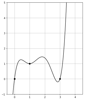
The polynomial jumps upwards immediately and strongly for $x > 3$.

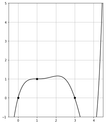
On the other hand, the plot of smoother_poly_with_degens() is given by

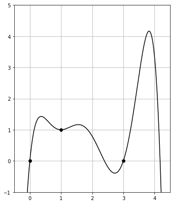
This stays in frame between $0$ and $4$, as desired.

Choose data to highlight and make the functions

This was enough to generate the functions for our paper. Actually, the three functions (in a total of six plots) in figures 1, 2, and 5 in our paper were hand chosen and hand-crafted for didactic purposes: the first two functions are simply a cubic and a quadratic with certain points labelled. The last function was the non-analytic-but-smooth semi-pathological counterexample, and so cannot be created through polynomial interpolation.

But the four functions highlighting different degenerate conditions in figures 3 and 4 were each created using this L2-minimizing interpolation system.

In particular, the function in figure 3 is

F3 = smoother_poly_with_degens(nc=1, residue_b=-3)

which is one of the simplest L2 minimizing polynomials with the typical Hermite conditions, $f''(c_0) = 0$, and opposite-default sign of $f'(b_0)$.

The three functions in figure 4 are (from left to right)

F_bmin = smoother_poly_with_degens(nc=1, nb=1, residue_c=10, residue_b=10)
F_bzero = smoother_poly_with_degens(nc=1, nb=2, residue_c=-20, residue_b=20)
F_bmax = smoother_poly_with_degens(nc=1, nb=1, residue_c=20, residue_b=-10)

We chose much larger residues because the goal of the figure is to highlight how the local behavior at those points corresponds to the behavior of the mean value abscissae, and larger residues makes those local behaviors more dominating.

Plotting all possible mean value abscissae

Now that we can choose our functions, we want to figure out how to find all solutions of the mean value condition $$ F(b, c) = \frac{f(b) - f(a_0)}{b - a_0} - f'(c). $$ Here I write $a_0$ as it's fixed, while both $b$ and $c$ vary.

Our primary interest in these solutions is to facilitate graphical experimentation and exploration of the problem — we want these pictures to help build intuition and provide examples.

Although this may seem harder, it is actually a much simpler problem. The function $F(b, c)$ is continuous (and roughly as smooth as $f$ is).

Our general idea is a common approach for this sort of problem:

1. Compute the values of $F(b, c)$ on a tight mesh (or grid) of points.
2. Restrict attention to the domain where solutions are meaningful.
3. Plot the contour of the $0$-level set.

Contours can be well-approximated from a tight mesh. In short, if there is a small positive number and a small negative number next to each other in the mesh of computed values, then necessarily $F(b, c) = 0$ between them. For a tight enough mesh, good plots can be made.

To solve this, we again have sympy create and compute the function for us. We use numpy to generate the mesh (and to vectorize the computations, although this isn't particularly important in this application), and matplotlib to plot the resulting contour.

Before giving code, note that the symbol F in the sympy code below stands for what we have been mathematically referring to as $f$, and not $F$. This is a potential confusion from our sympy-capitalization convention. It is still necessary to have sympy compute $F$ from $f$.

In code, this looks like

import sympy
import scipy
import numpy as np
import matplotlib.pyplot as plt

def abscissa_plot(F, n=300):
    # Compute the derivative of f
    DF = sympy.diff(F,X)

    # Define CAP_F — "capital F"
    #
    # this is (f(b) - f(0))/(b - 0) - f'(c).
    CAP_F = (F.subs(X, B) - F.subs(X, 0)) / (B - 0) - DF.subs(X, C)

    # build the mesh
    b1d = np.linspace(-.5, 4.5, n)
    b2d, c2d = np.meshgrid(b1d, b1d)

    # compute CAP_F within the mesh
    cap_f_mesh = sympy.lambdify((B, C), CAP_F)(b2d, c2d)

    # restrict attention to below the diagonal — we require c < b
    # (although the mas inequality looks reversed in this perspective)
    valid_cap_f_mesh = scipy.ma.array(cap_f_mesh, mask=c2d>b2d)

    # Set up plot basics
    fig = plt.figure(figsize=(6, 2.5))
    ax = fig.add_subplot(1, 1, 1)
    ax.set_aspect('equal')
    ax.grid(True)
    ax.set_xlim([-.5, 4.5])
    ax.set_ylim([-.5, 4.5])

    # plot the contour
    ax.contour(b2d, c2d, valid_cap_f_mesh, [0], colors='k')

    # plot a diagonal line representing the boundary
    ax.plot(b1d,b1d,'k–')

    # plot the guaranteed point
    ax.plot(b0,c0,'ko')

    fig.savefig("abscissa_plot.pdf")

Then plots of solutions to $F(b, c) = 0$ for our basic polynomials are given by

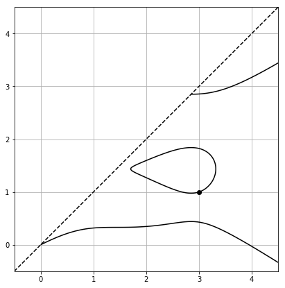
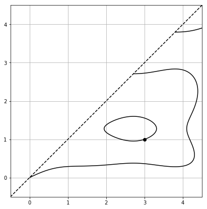
for poly_with_degens(), while for smoother_poly_with_degens() we get

And for comparison, we can now create a (slightly worse looking) version of the plots in figure 3.

F3 = smoother_poly_with_degens(nc=1, residue_b=-3)
basic_plot(F3)
abscissa_plot(F3)

This produces the two plots

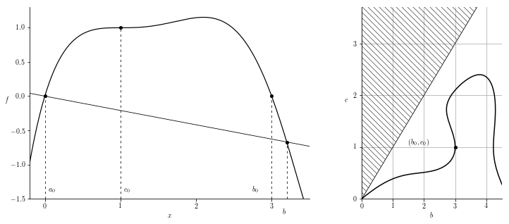
For comparison, a (slightly scaled) version of the actual figure appearing in the paper is

Copy of the code

A copy of the code used in this note (and correspondingly the code used to generate the functions for the paper) is available on my github as an ipython notebook.

Leave a comment

Comment via email