[This note is more about modeling some of the mathematics behind political events than politics themselves. And there are pretty pictures.]
Gerrymandering has become a recurring topic in the news. The Supreme Court of the US, as well as more state courts and supreme courts, is hearing multiple cases on partisan gerrymandering (all beginning with a case in Wisconsin).
Intuitively, it is clear that gerrymandering is bad. It allows politicians to choose their voters, instead of the other way around. And it allows the majority party to quash minority voices.
But how can one identify a gerrymandered map? To quote Justice Kennedy in his Concurrence the 2004 Supreme Court case Vieth v. Jubelirer:
When presented with a claim of injury from partisan gerrymandering, courts confront two obstacles. First is the lack of comprehensive and neutral principles for drawing electoral boundaries. No substantive definition of fairness in districting seems to command general assent. Second is the absence of rules to limit and confine judicial intervention. With uncertain limits, intervening courts–even when proceeding with best intentions–would risk assuming political, not legal, responsibility for a process that often produces ill will and distrust.
Later, he adds to the first obstacle, saying:
The object of districting is to establish “fair and effective representation for all citizens.” Reynolds v. Sims, 377 U.S. 533, 565—568 (1964). At first it might seem that courts could determine, by the exercise of their own judgment, whether political classifications are related to this object or instead burden representational rights. The lack, however, of any agreed upon model of fair and effective representation makes this analysis difficult to pursue.
From Justice Kennedy's Concurrence emerges a theme — a "workable standard" of identifying gerrymandering would open up the possibility of limiting partisan gerrymandering through the courts. Indeed, at the core of the Wisconsin gerrymandering case is a proposed "workable standard", based around the efficiency gap.
Thomas Schelling and Segregation
In 1971, American economist Thomas Schelling (who later won the Nobel Prize in Economics in 2005) published Dynamic Models of Segregation (Journal of Mathematical Sociology, 1971, Vol 1, pp 143–186). He sought to understand why racial segregation in the United States seems so difficult to combat.
He introduced a simple model of segregation suggesting that even if each individual person doesn't mind living with others of a different race, they might still choose to segregate themselves through mild preferences. As each individual makes these choices, overall segregation increases.
I write this post because I wondered what happens if we adapt Schelling's model to instead model a state and its district voting map. In place of racial segregation, I consider political segregation. Supposing the district voting map does not change, I wondered how the efficiency gap will change over time as people further segregate themselves.
It seemed intuitive to me that political segregation (where people who had the same political beliefs stayed largely together and separated from those with different political beliefs) might correspond to more egregious cases of gerrymandering. But to my surprise, I was (mostly) wrong.
Let's set up and see the model.
Schelling's Model
Let us first set up Schelling's model of segregation. Let us model a state as a grid, where each square on that grid represents a house. Initially ten percent of the houses are empty (White), and the remaining houses are randomly assigned to be either Red or Blue.
We suppose that each person wants to have a certain percentage ($p$) of their neighbors that are like itself. By "neighbor", we mean those in the adjacent squares. We will initially suppose that $p = 0.33$, which is a pretty mild condition. For instance, each person doesn't mind living with 66 percent of their neighbors being different, so long as there a couple of similar people nearby.
At each step (which I'll refer to as a year), if a person is unhappy (i.e. fewer than $p$ percent of their neighbors are like that person) then they leave their house and move randomly to another empty house. Notice that after moving, they may or may not be happy, and they will cause other people to perhaps become happy or become unhappy.
We also introduce a measure of segregation. We call the segregation the value of $$\text{segregation} = \frac{(\sum \text{number of same neighbors})}{(\sum \text{number of neighbors})},$$ summed across the houses in the grid, and where empty spaces aren't the same as anything, and don't count as a neighbor. Thus high segregation means that more people are surrounded only by people like them, and low segregation means people are very mixed. (Note also that 50 percent segregation is considered "very unsegregated", as it means half your neighbors are the same and half are different).
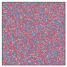
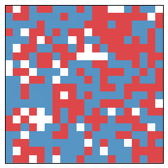
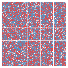
To get to a specific example, here is an instance of this model for $400$ spaces in a $20$ by $20$ grid.
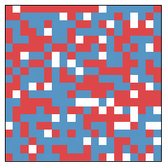
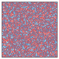
Initially, there is a lot of randomness, and segregation is a low $0.50$. After one year, the state looks like:
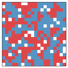
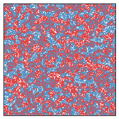
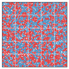
After another year, it changes a bit more:
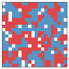
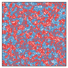
From year to year, the changes are small. But already significant segregation is occurring. The segregation measure is now at $0.63$. After another 10 years, we get the following picture:
That map appears extremely segregated, and now the segregation measure is $0.75$. Further, it didn't even take very long!
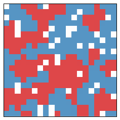
Let's look at a larger model. Here is a 200 by 200 grid. And since we're working larger, suppose each square "neighbors" the nearest 24, so that a neighborhood around 'o' looks like
xxxxx
xxxxx
xxoxx
xxxxx
xxxxx
Then we get:
Initially this looks quite a bit like red, white, and blue static. Going forward a couple of years, we get
Let us now fast forward ten years.
And after another ten years...
As an example of the sorts of things that can happen, we present several 15 second animations of these systems with a variety of initial parameters. In each animation, 30 years pass — one each half second.
We first consider a set of cases where we hold everything fixed except for how large people consider their "neighborhood." In the following, neighborhood sizes range from your nearest 8 neighbors (those which are 1 step away, counting diagonal steps) to those which are up to 5 steps away. The behavior is a bit different in each one. Note that in the really-large neighborhood case, there are only a few people moving at all.
We next consider the cases when people want to have neighborhoods which are at least 40 percent like themselves. That is, people want to cluster a bit more. The list then spans over differing neighborhood sizes again.
These are stunning, and sort of beautiful. I am reminded of slime mold growth.
We now up percentage again to $p = 0.5$. That is, people only feel comfortable in neighborhoods with at least 50 percent of occupants similar to themselves. This is actually the parameter that Schelling introduced in his paper and experiments.
The higher comfort factor leads to much quicker convergence to extreme segregation. This is intuitive — high individual segregation concerns leads to quick societal segregation.
We now increase the population to a million people. In the first animation, there is large segregation at the end, but it manifests as a sort of network of red and blue wispy fingers rather than big blobs. Partly this is because there simply more room. But it's also a manifestation of the fact that with small neighborhood sizes, one gets mostly local effects.
The second and third animations are pretty astounding to me. In these, people want 40 percent similarity with their neighbors, and their "neighborhoods" are those without four steps (including diagonally) to them. In the third, 55% of the population is Red and 45% is Blue. In the last one, a much larger majority is Red, and there are so few Blue people that they are all rapidly moving trying to find some base where they feel comfortable. But they never found a comfort base.
Disclaimer
We should take a moment to say what it is that we are actually trying to measure. Is this supposed to be a perfect model of actual behavior? No.
This note has been examining how some individual incentives, decisions, and perceptions of difference can lead collectively towards greater segregation. Although I have phrased this in terms of political party identification, this analysis is so abstract that it could be applied to any singular distinction.
We should also note that several causes of segregation are omitted from consideration. One is organized action (be is legal or illegal, in good faith or in bad). Another are economic causes behind many separations, such as how the poor are separated from the rich, the unskilled from the skilled, the less educated from the more educated. These lead to separations in job, pastime, residence, and so on. And as political party affiliation correlates strongly with income, and income correlates strongly with where one lives, this is a major factor to omit.
I do not claim that these other sources of discrimination and segregation are less important, but only that I do not know how to model them. And instead I follow Schelling's line of thought, whereby one looks to see to what extent we might expect individual action to lead to collective outcomes.
Altering Schelling to Model Voting Districts
Given a Schelling model, we now adapt it incorporate voting districts. Let us suppose that our square is divided up into (regular rectangular) regions of voters. We will assume a totally polarized voter base, so that Red people will always vote for the Red party and Blue people will always vote for the Blue party. (This is a pretty strong assumption).
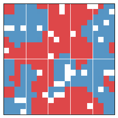
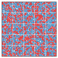
Before we describe exactly how we set up the model, let's look at an example. Given a typical Schelling model, we separate it into (in this case, 10) districts.
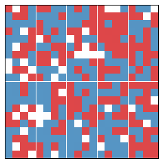
Each of the 10 areas vote, giving some tallies. In this case, we have the following table which describes the results of this year's vote. Districts are numbered from top left to bottom right, sequentially.
| District | Blue Vote | Red Vote | Winner | Blue Wasted | Red Wasted | Net Wasted |
|---|---|---|---|---|---|---|
| 0 | 18 | 14 | blue | 3 | 14 | -11 |
| 1 | 20 | 16 | blue | 3 | 16 | -13 |
| 2 | 19 | 15 | blue | 3 | 15 | -12 |
| 3 | 12 | 25 | red | 12 | 12 | 0 |
| 4 | 18 | 20 | red | 18 | 1 | 17 |
| 5 | 19 | 15 | blue | 3 | 15 | -12 |
| 6 | 21 | 13 | blue | 7 | 13 | -6 |
| 7 | 23 | 15 | blue | 7 | 15 | -8 |
| 8 | 22 | 15 | blue | 6 | 15 | -9 |
| 9 | 14 | 23 | red | 14 | 8 | 6 |
"Blue Wasted" refers to a wasted blue vote (similarly for Red). This is a key idea counted in the efficiency gap, and contributes towards the overall measure of gerrymandering.
A wasted vote is one that doesn't contribute to winning an additional election. A vote can be wasted in two different ways. All votes for a losing candidate are wasted, since they didn't contribute to a win. On the other hand, excess voting for a single candidate is also wasted.
So in District 0, the Blue candidate won and so all 14 Red votes are wasted. The Blue candidate only needed 15 votes to win, but received 18. So there are three excess Blue votes, which means that there are 3 Blue votes wasted.
I adopt that convention (for ease of summing up) that the net wasted votes is the number of Blue wasted votes minus the number of Red wasted votes. So if it is positive, this means that more Blue votes were wasted than Red. And if it's negative, then more Red votes were wasted than Blue.
Aside: How the Efficiency Gap measures Gerrymandering
With this example in mind, a rough definition of gerrymandering in a competitive district is to draw lines so that one party has many more wasted votes. In this example, there are 186 Blue voters and 171 Red voters, so it might be expected that approximately half of the winners would be Red and half would be Blue. But in fact there are 7 Blue winners and only 3 Red winners.
And a big reason why is that the overall net wasted number of votes is $-48$, which means that $48$ more Red votes than Blue votes did not contribute to a winning election.
So roughly, more wasted votes corresponds to more gerrymandering. The efficiency gap is defined to be
$$ \text{Efficiency Gap} = \frac{\text{Net Wasted Votes}}{\text{Number of Voters}}.$$
In this case, there are $48$ wasted votes and $357$ voters, so the efficiency gap is $48/357 = 0.134$. This number, 13.4 percent, is very high. The proposed gap to raise flags in gerrymandering cases is 7 percent — any higher, and one should consider redrawing district lines.
The efficiency gap is extremely easy to compute, which is a good plus. But whether it is a good indicator of gerrymandering is more complicated, and is one of the considerations in teh Supreme Court case concerining gerrymandering in Wisconsin.
A More Complete Description of the Model
With this example in mind, we are now prepared to describe the model explicitly. The initial setup is the same as in Schelling's model. A state is a rectangular grid, where each square on this grid represents a house. Unoccupied houses are White. If a Red person occupies a house, then the house is colored Red. If a Blue person occupies a house, then that house is colored Blue. Each year, all the Red people vote for the Red candidate, and all Blue people vote for the Blue candidate, and we can tally the results. We will then measure the efficiency gap.
At the same time, each year people may move as in Schelling's model. A person is satisfied if they have at least $p$ percent of their neighbors which are similar to them. We will again default to $33$ percent, and a person's neighbors will be all those people which adjacent (or for larger models, perhaps 2-step adjacent, or that flavor) away.
At each step, we can measure the segregation (which we know will increase from Schelling's model) and the efficiency gap.
At last, we are prepared to investigate the relationship between segregation and the efficiency gap.
Simulations
In our first simulation, there is an initial segregation of 51% and and initial efficiency gap of 6%. This is pictured below.
As we can see, an increase in segregation corresponds to an increase in the efficiency gap. 1 1This was honestly the first simulation I did, and I was generically pleased that my expectation was working out. But as we shall see, this pattern does not hold up.
Let us now consider a second simulation. There are no parameters changed between this and the above simulation, aside from the chance placement of people.

An increase in segregation actually occurs with a decrease in efficiency gap. Further, if we stepped through year to year, we would see that as the state became more segregated, it also lowered its efficiency gap.
At least naively we should no longer expect increased segregation to correspond to an increase in the efficiency gap.
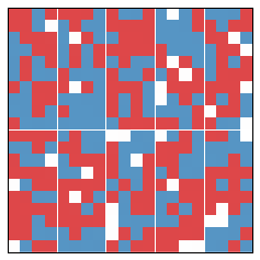
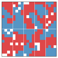
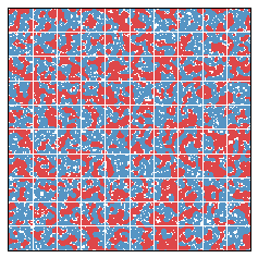
Let's try a larger simulation. This one is 200 x 200, with 25 districts.
Again, segregation correlates negatively with the efficiency gap.
What if 55 percent of the population is blue? Does this imbalance lead to interesting simulations? We present two such simulations below.

In each of these simulations, there was an initially large efficiency gap. This is fundamentally caused by the relatively equidistributed Red minority, which essentially loses everywhere. We might say that the Red group begins in a cracked state. After 20 years, the efficiency gap falls, since segregation has the interesting side effect of relieving the Red people from their diffused state.
In fact I ran a very large number of simulations with a variety of parameters, and generically increased segregation tends to correspond to a decrease in the efficiency gap.
Result: Segregation Correlates (Weakly) Negatively with Efficiency Gap
More segregation leads to a smaller efficiency gap. Why might this be?
I think one of the major reasons is evident in the last pair of simulations I presented above. Uniform segregation reduces the "cracking" gerrymandering technique. In cracking, one tries to divide a larger group into many smaller minorities by splitting them into many districts. This maximizes the number of wasted votes coming from lost elections (as opposed to wasted votes from packing lots of people into one district so that they over-win an election). Segregation produces clusters, and these clusters tend to win their local district's election.
The few examples above where high segregation accompanied high efficiency gaps were when the segregated clusters happened to be split by district lines.2 2Excitingly, this is contrary to my expectations. Erasmus Darwin, the grandfather of Charles Darwin (and biologist Francis Galton) had a theory that every once in a while, one should perform a ridiculous experiment. It essentially always fails, but when it works it's absolutely terrific. Darwin played the trombone to his tulips. The result of this particular experiment (and the result in this note) was negative. (story from Littlewood's Mathematicians Miscellany)
Works Referenced
I read many pieces from others while preparing this post. Though I don't cite any of them explicitly, these works were essential for my preparation.
- A formula goes to court: partisan gerrymandering and the effiency gap. By Mira Bernstein and Moon Duchin. Available on the arXiv.
- An impossibility theorem for gerrymandering. By Boris Alexeev and Dustin Mixon. Available on the arXiv.
- Flaws in the efficiency gap. By Christopher Chambers, Alan Miller, and Joel Sobel. Available on Christopher Chambers' site.
- How the new math of gerrymandering Works, in the New York Times. By Nate Cohn and Quoctrung Bui. Available at the nytimes.
- The flaw in America's 'holy grail' against gerrymandering, in the Atlantic. By Sam Kean. Available at the atlantic.
- Dynamic Models of Segregation, by Thomas Schelling. In Journal of Mathematical Sociology, 1971, Vol 1, pp143–186.
Code
Below, I include the code I used to generate these simulations and images. This code, as well as much of the code I used to generate the particular data above, is available as a jupyter notebook in my github. (But I would mention that unlike some previous notebooks I've made available, this was really a working notebook and isn't a final product in itself).
Code for Schelling Plots
The heart of this code is based on code from Allen Downey, presented in his book "Think Complexity." He generously released his code under the MIT license.
"""
Copyright (c) 2018 David Lowry-Duda

Permission is hereby granted, free of charge, to any person obtaining a copy
of this software and associated documentation files (the "Software"), to deal
in the Software without restriction, including without limitation the rights
to use, copy, modify, merge, publish, distribute, sublicense, and/or sell
copies of the Software, and to permit persons to whom the Software is
furnished to do so, subject to the following conditions:

The above copyright notice and this permission notice shall be included in all
copies or substantial portions of the Software.

THE SOFTWARE IS PROVIDED "AS IS", WITHOUT WARRANTY OF ANY KIND, EXPRESS OR
IMPLIED, INCLUDING BUT NOT LIMITED TO THE WARRANTIES OF MERCHANTABILITY,
FITNESS FOR A PARTICULAR PURPOSE AND NONINFRINGEMENT. IN NO EVENT SHALL THE
AUTHORS OR COPYRIGHT HOLDERS BE LIABLE FOR ANY CLAIM, DAMAGES OR OTHER
LIABILITY, WHETHER IN AN ACTION OF CONTRACT, TORT OR OTHERWISE, ARISING FROM,
OUT OF OR IN CONNECTION WITH THE SOFTWARE OR THE USE OR OTHER DEALINGS IN THE
SOFTWARE.
"""

import numpy as np
import matplotlib.pyplot as plt

from matplotlib import animation
from matplotlib.colors import LinearSegmentedColormap
from scipy.signal import correlate2d

class Schelling:
    """A 2D grid of Schelling agents."""
    options = dict(mode='same', boundary='wrap')

    def __init__(self, n, m=None, p=0.5, empty_prob=0.1, red_prob=0.45, size=3):
        """
        Initialize grid with attributes.

        Args:
            n: (int) number of rows.
            m: (int) number of columns. In None, defaults to n.
            p: (float) ratio of neighbors that makes one feel comfortable.
            empty_prob: (float) probability an initial cell is empty.
            red_prob: (float) probability an initial cell is Red.
            size: (odd int) size of the neighborhood kernel.
        """
        self.p = p
        m = n if m is None else m
        EMPTY, RED, BLUE = 0, 1, 2
        empty_prob = 0.1
        choices = [EMPTY, RED, BLUE]
        probs = [empty_prob, red_prob, 1 - empty_prob - red_prob]
        self.array = np.random.choice(choices, (n, m), p=probs).astype(np.int8)
        self.kernel = self._make_kernel(size)

    def _make_kernel(self, size):
        """
        Construct size*size adjacency kernel.

        Args:
            size: (int) for size of kernel.

        Returns:
            np.array such as (for size=3)

            [[1,1,1],
             [1,0,1],
             [1,1,1]]

            In the size=n case, it's an n*n array of ones with a zero at
            the center.
        """
        pad = int((size**2-1)/2)
        return np.array([1]*(pad) + [0] + [1]*(pad)).reshape((size,size))

    def count_neighbors(self):
        """
        Surveys neighbors of cells.

        Returns:
            This returns the tuple (occupied, frac_red, frac_same)
            where

            occupied: logical array indicating occupied cells.
            frac_red: array containing fraction of red neighbors around each cell.
            frac_same: array containing the fraction of similar neighbors.

        Note:
            Unoccupied cells do not count in neighbors or similarity.
        """
        a = self.array
        EMPTY, RED, BLUE = 0, 1, 2

        # These create np.arrays where each entry is True if condition is true
        red = a==RED
        blue = a==BLUE
        occupied = a!=EMPTY

        # count red neighbors and all neighbors
        num_red = correlate2d(red, self.kernel, **self.options)
        num_neighbors = correlate2d(occupied, self.kernel, **self.options)

        # compute fraction of similar neighbors
        frac_red = num_red / num_neighbors
        frac_blue = 1 - frac_red
        frac_same = np.where(red, frac_red, frac_blue)

        # no neighbors is considered the same as no similar neighbors
        frac_same[num_neighbors == 0] = 0
        frac_red[num_neighbors == 0] = 0

        # Unoccupied squares are not similar to anything
        frac_same[occupied == 0] = 0

        return occupied, frac_red, frac_same

    def segregation(self):
        """Computes the average fraction of similar neighbors."""
        occupied, _, frac_same = self.count_neighbors()
        return np.sum(frac_same) / np.sum(occupied)

    def step(self):
        """Executes one time step."""
        a = self.array

        # find the unhappy cells
        occupied, _, frac_same = self.count_neighbors()
        unhappy_locs = locs_where(occupied & (frac_same < self.p))

        # find the empty cells
        empty = a==0
        num_empty = np.sum(empty)
        empty_locs = locs_where(empty)

        # shuffle the unhappy cells
        if len(unhappy_locs):
            np.random.shuffle(unhappy_locs)

        # for each unhappy cell, choose a random destination
        for source in unhappy_locs:
            i = np.random.randint(len(empty_locs))
            dest = tuple(empty_locs[i])

            # move
            a[dest] = a[tuple(source)]
            a[tuple(source)] = 0
            empty_locs[i] = source

        num_empty2 = np.sum(a==0)
        assert num_empty == num_empty2
        return

def locs_where(condition):
    """
    Find cells where a logical array is True.

    Args:
        condition: (2D numpy logical array).

    Returns:
        Array with one set of coordinates per row indicating where
        condition was true.

    Example:
        Input is (as np.array)

        [[1,0],
         [1,1]]

        Then the output will be

        [[0,0],[1,0],[1,1]]

        which are the three locations of the nonzero (True) cells.
    """
    return np.transpose(np.nonzero(condition))


def make_cmap(color_dict, vmax=None, name='mycmap'):
    """
    Makes a custom color map.

    Args:
        color_dict: (dict) of form {number:color}.
        vmax: (float) high end of the range. If None, use max value
              from color_dict.
        name: (str) name for map.

    Returns:
        pyplot color map.
    """
    if vmax is None:
        vmax = max(color_dict.keys())
    colors = [(value/vmax, color) for value, color in color_dict.items()]
    cmap = LinearSegmentedColormap.from_list(name, colors)
    return cmap


class SchellingViewer:
    """Generates animated view of Schelling array"""

    # colors from http://colorbrewer2.org/#type=diverging&scheme=RdYlBu&n=5
    colors = ['#fdae61','#abd9e9','#d7191c','#ffffbf','#2c7bb6']
    cmap = make_cmap({0:'white', 1:colors[2], 2:colors[4]})

    options = dict(interpolation='none', alpha=0.8)

    def __init__(self, viewee):
        """
        Initialize.

        Args:
            viewee: (Schelling) object to view
        """
        self.viewee = viewee
        self.im = None
        self.hlines = None
        self.vlines = None

    def step(self, iters=1):
        """Advances the viewee the given number of steps."""
        for i in range(iters):
            self.viewee.step()

    def draw(self, grid=False):
        """
        Draws the array, perhaps with a grid.

        Args:
            grid: (boolean) if True, draw grid lines. If False, don't.
        """
        self.draw_array(self.viewee.array)
        if grid:
            self.draw_grid()

    def draw_array(self, array=None, cmap=None, **kwds):
        """
        Draws the cells.

        Args:
            array: (2D np.array) Array to draw. If None, uses self.viewee.array.
            cmap: colormap to color array.
            **kwds: keywords are passed to plt.imshow as options.
        """
        # Note: we have to make a copy because some implementations
        # of step perform updates in place.
        if array is None:
            array = self.viewee.array
        a = array.copy()
        cmap = self.cmap if cmap is None else cmap

        n, m = a.shape
        plt.axis([0, m, 0, n])
        # Remote tickmarks
        plt.xticks([])
        plt.yticks([])

        options = self.options.copy()
        options['extent'] = [0, m, 0, n]
        options.update(kwds)
        self.im = plt.imshow(a, cmap, **options)

  def draw_grid(self):
       a = self.viewee.array
       n, m = a.shape
       lw = 2 if m < 10 else 1
       options = dict(color='white', linewidth=lw)
       rows = np.arange(1, n)
       self.hlines = plt.hlines(rows, 0, m, **options)
       cols = np.arange(1, m)
       self.vlines = plt.vlines(cols, 0, n, **options)

  def animate(self, frames=20, interval=200, grid=False):
      """
      Creates an animation. Args: frames: (int) number of frames to draw.
      interval: (int) time between frames in ms. grid: (boolean) if True, include
      grid in drawings.
      """
      fig = plt.figure()
      self.draw(grid=grid)
      anim = animation.FuncAnimation(fig, self.animate_func,
                init_func=self.init_func, frames=frames, interval=interval)
      return anim

  def init_func(self):
      """Called at the beginning of an animation."""
      pass

  def animate_func(self, i):
      """Draws one frame of the animation."""
      if i > 0:
          self.step()
          a = self.viewee.array
          self.im.set_array(a)
          return (self.im,)
Then a typical Schelling object can be viewed through a call like
grid = Schelling(n=6)
viewer = SchellingViewer(grid)
viewer.draw(grid=True)
Code for District Plots
And code for the District analysis, which sits on top of Schelling from above.
class Districts(Schelling):
    """A 2D grid of Schelling agents organized into districts."""

    def __init__(self, n, m=None, p=0.5, rows=2,
                 cols=2, empty_prob=0.1, red_prob=0.45, size=3):
        """
        Initialize grid.

        Args:
            n: (int) number of rows in grid.
            m: (int) number of columns in grid. If None, defaults to n.
            p: (float) ratio of neighbors required to feel comfortable.
            rows: (int) number of rows of districts.
            cols: (int) number of columns of districts.
            empty_prob: (float) probability each initial cell is empty.
            red_prob: (float) probability each initial cell is Red.
            size: (odd int) size of neighborhood kernel.

        Note:
            `rows` must divide n, and `cols` must divide m.
            An exception is raised otherwise.
        """
        self.p = p
        self.n = n
        self.m = n if m is None else m
        self.rows = rows
        self.cols = cols
        self.schelling_grid = Schelling(n, m=self.m, p=p,
                                        empty_prob=empty_prob,
                                        red_prob=red_prob, size=3)
        self.array = self.schelling_grid.array
        self.kernel = self.schelling_grid.kernel
        self.row_mult = self.n//self.rows
        self.col_mult = self.m//self.cols
        try:
            assert(self.row_mult*self.rows==self.n)
            assert(self.col_mult*self.cols==self.m)
        except AssertionError:
            raise Exception(("The number of rows and number of columns must"
                             " divide the size of the grid."))
        self.districts = self.make_districts()

    def make_districts(self, array=None):
        """
        Returns array of np.arrays, one for each district.
        """
        if array is None:
            array = self.array
        # double indices works from numpy sugar
        return [array[self.row_mult*i: self.row_mult*(i+1),
                      self.col_mult*j: self.col_mult*(j+1)]
                for i in range(self.rows) for j in range(self.cols)]

    def votes(self, output=False):
        """Count votes in each district."""
        votes = dict()
        if output:
            print ("Vote totals\n———–\n")
        for num, district in enumerate(self.districts):
            IS_RED = 1
            IS_BLUE = 2
            votes[num] = {'red': list(district.flatten()).count(IS_RED),
                          'blue': list(district.flatten()).count(IS_BLUE)}
            if output:
                print ("District {}::   Red vote: {},   Blue vote: {}".format(
                        num, votes[num]['red'], votes[num]['blue']))
        return votes

    def tally_votes(self, output=False):
        """Detect winners from votes in each district."""
        tallies = self.votes()
        if output:
            print ("Tallying votes\n————–\n")
        for num, district in enumerate(self.districts):
            dist_tally = tallies[num]
            dist_tally.update(self.determine_winner(dist_tally))
        return tallies

    def determine_winner(self, vote_tally):
        """
        Given a single district's vote_tally, determine the winner.

        Returns:
            A dictionary with the keys

            'winner'
            'red_wasted'
            'blue_wasted'

            computed from vote tally.
        """
        res = dict()
        if vote_tally['red'] > vote_tally['blue']:
            res['winner'] = 'red'
            res['red_wasted'] = vote_tally['red'] - vote_tally['blue'] - 1
            res['blue_wasted'] = vote_tally['blue']
        elif vote_tally['blue'] > vote_tally['red']:
            res['winner'] = 'blue'
            res['blue_wasted'] = vote_tally['blue'] - vote_tally['red'] - 1
            res['red_wasted'] = vote_tally['red']
        else:
            res['winner'] = 'tie'
            res['red_wasted'] = 0
            res['blue_wasted'] = 0
        return res

    def net_wasted_votes_by_district(self):
        """
        Compute net wasted votes in each district.

        Note:
            We adopt the convention that 1 wasted vote means a wasted blue vote,
            while -1 wasted vote means a wasted red vote.
        """
        res = dict()
        tallies = self.tally_votes()
        for num, district in enumerate(self.districts):
            res[num] = tallies[num]['blue_wasted'] - tallies[num]['red_wasted']
        return res

    def net_wasted_votes(self):
        wasted_by_dist = self.net_wasted_votes_by_district()
        return sum(wasted_by_dist[num] for num in wasted_by_dist.keys())

    def efficiency_gap(self):
        return abs(self.net_wasted_votes()) / (np.sum(self.array != 0))

    def votes_to_md_table(self):
        """
        Output votes to a markdown table.

        This is a jupyter notebook convenience method.
        """
        vote_tally = self.tally_votes()
        ret = "|District|Blue Vote|Red Vote|Winner|Blue Wasted|Red Wasted|Net Wasted|\n"
        ret += "|-|-|-|-|-|-|-|\n"
        for i in range(len(vote_tally)):
            district = i
            dist_res = vote_tally[i]
            bv = dist_res['blue']
            bw = dist_res['blue_wasted']
            rv = dist_res['red']
            rw = dist_res['red_wasted']
            nw = bw - rw
            winner = dist_res['winner']
            ret += "|{}|{}|{}|{}|{}|{}|{}|\n".format(district, bv, rv, winner, bw, rw, nw)
        return ret


class District_Viewer(SchellingViewer):
    """Viewer of Schelling District arrays"""

    def __init__(self, districts):
        super().__init__(districts.schelling_grid)
        self.row_multiplier = districts.row_mult
        self.col_multiplier = districts.col_mult

    def draw_grid(self):
        """Draws the grid."""
        a = self.viewee.array
        n, m = a.shape
        lw = 2 if m < 10 else 1
        options = dict(color='white', linewidth=lw)

        rows = self.row_multiplier*np.arange(1, n)
        self.hlines = plt.hlines(rows, 0, m, **options)

        cols = self.col_multiplier*np.arange(1, m)
        self.vlines = plt.vlines(cols, 0, n, **options)
The functionality is built on top of Schelling, above. Typical use would look like
dgrid = Districts(10, cols=5, p=.2)
viewer = District_Viewer(dgrid)
viewer.draw(grid=True)
dgrid.tally_votes()
Info on how to comment
To make a comment, please send an email using the button below. Your email address won't be shared (unless you include it in the body of your comment). If you don't want your real name to be used next to your comment, please specify the name you would like to use. If you want your name to link to a particular url, include that as well.
bold, italics, and plain text are allowed in comments. A reasonable subset of markdown is supported, including lists, links, and fenced code blocks. In addition, math can be formatted using
$(inline math)$or$$(your display equation)$$.Please use plaintext email when commenting. See Plaintext Email and Comments on this site for more. Note also that comments are expected to be open, considerate, and respectful.