mixedmath

Quanta Magazine and Alex Kontorovich recently published an explanation of key ideas in the Langlands Program. Alex narrates a video explanation as well.

A little while ago, Emily from Quanta Magazine asked if I could make some visualizations of modular forms and elliptic curves for this video.^{1 1}I should emphasize that I only made visualizations of the modular forms. The illustrations and aesthetic storytelling in this video all come from the incredible illustrator team at Quanta. I'd like to describe a few different aspects about these modular forms.

Four specific modular forms appear in the video. These are

1. The Ramanujan discriminant function
2. The modular form associated to the elliptic curve $Y^2 = X^3 + X + 17$
3. A weight $0$ Maass form with parameter $R \approx 20.10669$
4. The modular form 163.3.b.a.

Each of the above links is to a page in the L-Function and Modular Form database (LMFDB), which contains further information. I included the Maass form because I've devoted a lot of time recently to computing and verifying Maass forms.

The Delta function

How does one visualize a modular form? In my paper Visualizing Modular Forms,^{2 2}or the arxiv preprint 2002.05234

I compared and contrasted different methods of visualizing modular forms. For the Quanta video, I made high fidelity phaseplots.

To understand better how these visualizations are made, we'll create a visualization of the Ramanujan discriminant modular form $\Delta(z)$. To do this, we'll use Sage9.6+,^{3 3}This is a very recent build of sage. Older versions can make variants, but not phasemaps and not with different colormaps. which includes many of my complex plotting routines.

The first task is to compute $\Delta(z)$. This modular form has the equation \begin{equation*} \Delta(z) = e^{2 \pi i z} \prod_{n \geq 1} (1 - e^{2 \pi i n z})^{24}, \end{equation*} which can be approximated by the power series \begin{equation*} \Delta(z) \approx q - 24 q^2 + 252 q^3 - 1472 q^4 + \cdots \qquad (q = e^{2 \pi i z}). \end{equation*} In sage, we can compute this via

import cmath

delta_coeffs = [
  0, 1, -24, 252, -1472, 4830, -6048, -16744, 84480, -113643, -115920,
  534612, -370944, -577738, 401856, 1217160, 987136, -6905934, 2727432,
  10661420, -7109760, -4219488, -12830688, 18643272, 21288960, -25499225,
  13865712, -73279080, 24647168, 128406630, -29211840, -52843168, -196706304
]

def deltafn(z):
    """
    Compute an approximation to the delta function at z using the first few
    coefficients.

    For example, `deltafn(I)` should be approximately 0.001785
    """
    value = 0
    for idx, coeff in enumerate(delta_coeffs):
        value += coeff * cmath.exp(2 * cmath.pi * 1j * idx * z))
        # cmath does relatively quick, somewhat precise computation
    return value

print(deltafn(I))  # 0.00178374663460090

This modular form is particularly important in the history of modular forms, and thus sage actually knows how to compute the coefficients. For example, $\Delta(q)$ (in $q$-coordinates) can be computed in sage via

delta_qexp()

# prints the list of coefficients used above, omitting the initial 0
print(delta_qexp(30).coefficients())

This allows a low-precision approximation of $\Delta(z)$ at any point $z$ in the upper halfplane $\mathcal{H} = \{ z : \mathrm{Im} z > 0 \}$. For example,

P = complex_plot(
      deltafn, (-1, 1), (0.001, 1),
      cmap="magma", dark_rate=0, contoured=True,
      plot_points=300, aspect_ratio=1
)
P.show(axes=False)

generates the image

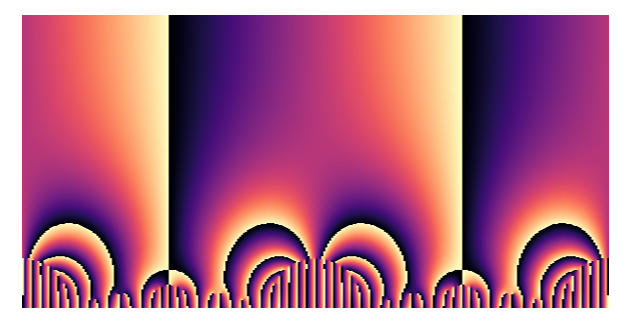
This uses the magma colormap in python's matplotlib library. Setting contoured=True and dark_rate=0 creates a pure phaseplot — only the phase is shown. This is computed on a $300 \times 300$ grid, which (depending on your computer) can take a little bit.

The visualizations for Quanta are shown on a disk model of the upper half-plane. In order to make these plots, we use the Cayley-type transform \begin{equation*} z \mapsto \frac{1 - iz}{z - i}, \end{equation*} which maps the unit disk to the $\mathcal{H}$. In particular, this maps $-i$ to $0$, $0$ to $i$, and $i$ to $i\infty$. In code, this is

def DtoH(z):
    """
    Map points on the Poincare disk to the upper half-plane.
    """
    return (1 - 1j*z)/(z - 1j)

Then we make a plot withcomplex_plot masks away NaN values. Setting values outside the unit circle to be +Infinity has the effect of making them white.

P = complex_plot(
    lambda x: +Infinity if abs(x) >= 0.99 else deltafn(DtoH(x)),
    (-1,1), (-1,1),
    cmap="magma", dark_rate=0, contoured=True,
    plot_points=300, aspect_ratio=1
)
P.show(axes=False)

makes the plot

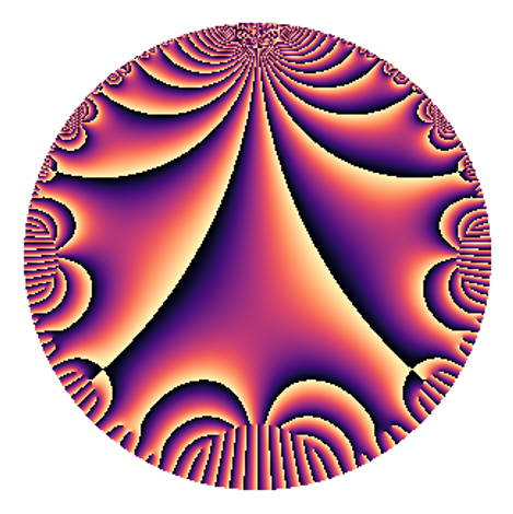
This is a low resolution, low fidelity version of the plot of the delta function appearing around 3:10 into the Quanta video (and it's rotated by 90 degrees).

The version for the video was computed with higher precision at higher resolution. To compute at higher precision, one can either use more coefficients or use the modularity of $\Delta(z)$. For the video I used only $50$ coefficients, but I only computed $\Delta(z)$ on the fundamental domain (where $50$ coefficients is enough to give high accuracy). See this answer on Math.StackExchange for another description of using modularity to achieve high fidelity. This code is taken from there. I actually don't perform these computations in sage, so this is lightly modified pure python version taken from a different application. The ideas are the same.

One way to do this is as follows.

def in_fund_domain(z):
    x = z.real()
    y = z.imag()
    if x < -0.51 or x > 0.51:
        return False
    if x*x + y*y < 0.99:
        return False
    return True

def act(gamma, z):
    a, b, c, d = gamma
    return (a*z + b) / (c*z + d)

def mult_matrices(mat1, mat2):
    a, b, c, d = mat1
    A, B, C, D = mat2
    return [a*A + b*C, a*B + b*D, c*A + d*C, c*B + d*D]

Id = [1, 0, 0, 1]

def pullback(z):
    """
    Returns gamma, w such that gamma(z) = w and w is
    (essentially) in the fundamental domain.
    """
    z = CDF(z)
    gamma = Id
    count = 1
    while not in_fund_domain(z):
        if (count > 1000): print(z, count)
        count += 1
        x, y = z.real(), z.imag()
        xshift = -floor(x + 0.5)
        shiftmatrix = [1, xshift, 0, 1]
        gamma = mult_matrices(shiftmatrix, gamma)
        z = act(shiftmatrix, z)
        if x*x + y*y < 0.99:
            z = -1/z
            gamma = mult_matrices([0, -1, 1, 0], gamma)
    return gamma, z

def smart_compute(z):
    gamma, z = pullback(DtoH(z))
    a, b, c, d = gamma
    return (-c*z + a)**12 * deltafn(z)

We can then produce a more accurate visualization.

P = complex_plot(
    lambda x: +Infinity if abs(x) >= 0.99 else smart_compute(x),
    (-1,1), (-1,1),
    cmap="magma", dark_rate=0, contoured=True,
    plot_points=300, aspect_ratio=1
)
P.show(axes=False)

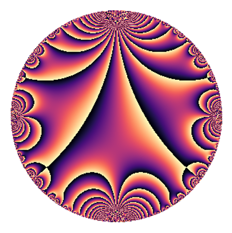
Notice how this completely removes the banding errors on the boundary. The remaining problems are due to resolution. The version in the video was computed using $4000$ plot points in a custom colormap. The render took approximately 40 minutes to complete.

Comments on the other functions

The other modular forms were each trickier to compute.

The modular form associated to the elliptic curve $Y^2 = X^3 + X + 17$ has conductor $124912$, which is too large to be included in the LMFDB. In practice, the underlying automorphisms of the modular group are much more annoying to work with as well. I set a long, "dumb" computation running ($300$ coefficients on $4000$ plot points, again downsampling in the end) and began to play around with methods of performing the computation more efficiently. But the long computation won.

I've computed this Maass form before. In fact, this is the same Maass form that appeared in this talk I gave. I think it's particularly beautiful. I'll write much more about Maass forms in the future. I also intend on creating new Maass form visualizations on the LMFDB later this year.

It was a fun challenge to visualize the "impossible modular form", i.e. the "counterexample to Fermat's Last Theorem" (appearing in the video near 11:05). I drew inspiration from the various honest mistakes I've made in visualizations over the last couple of years — plotting true modular forms with respect to the incorrect coordinates gives obviously structured forms a psychadelic look. See the mistakes from my first talk on visualizing modular forms back in 2019.

There are three common and natural coordinate choices for modular forms. There are coordinates in $\mathcal{H}$, coordinates in the unit disk (related by the Cayley-like transform to coordinates in $\mathcal{H}$), and $q$-coordinates (with respect to $q = e^{2 \pi i z}$.

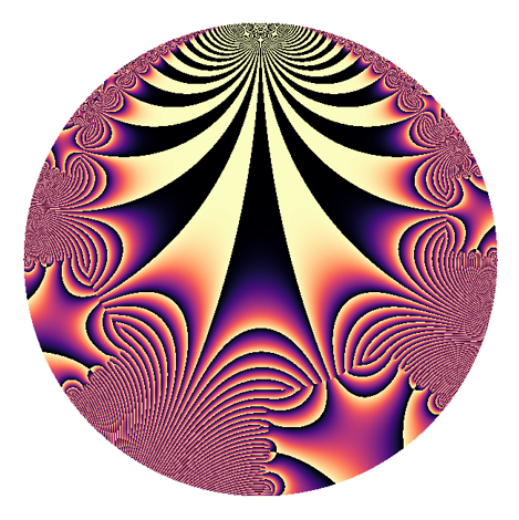
Morally, to make the "impossible modular form", I treated $q$-coordinates as if they were $\mathcal{H}$-coordinates and designed a domain coloring that was very incongruent around $0$. Let's make a similar map for $\Delta(z)$.

# Relationships between the three standard bases
DtoH = lambda x: (-CDF.0*x + 1)/(x - CDF.0)
Htoq = lambda x: exp(2 * CDF.pi() * CDF.0 * x)
Dtoq = lambda x: Htoq(DtoH(CDF(x)))

P = complex_plot(
  # deltafn expects DtoH(x), *not* Dtoq(x)
  lambda x: +Infinity if abs(x) >= 0.99 else deltafn(Dtoq(x)),
  (-1,1), (-1,1),
  cmap="magma", dark_rate=0, contoured=True,
  plot_points=600, aspect_ratio=1
)
P.show(axes=False)

I increased the number of points a bit, but this makes the following.

The actual modular form used for this was a distinguished modular form. It's the modular form with Fourier coefficients $a(n^2) = n^2$ for all $n^2 < 41$, and $a(p) = 0$ for $p < 41$. The the first several coefficients are the typical squares. That this modular form exists and is of level $163$ is numerologically related to other Ramanujan conjectures.

Leave a comment

Comment via email