mixedmath

In my previous note, we considered equidistribution of rational points on the circle $X^2 + Y^2 = 2$. This is but one of a large family of equidistribution results + that + I'm not particularly familiar with.

This note is the first in a series of notes dedicated to exploring this type of equidistribution visually. In this note, we will investigate a simpler case — rational points on the line.

We know that $\mathbb{Q}$ is dense in $\mathbb{R}$. An equidistribution statement is roughly a way of quantifying this density. Let $I \subseteq \mathbb{R}$ be a finite interval. We will say that a sequence ${x_n}_{n \geq 1}$ of elements $x_n \in I$ is $\mu$-equidistributed on $I$ (or equidistributed with respect to $\mu$) if for each subinterval $J \subset I$ we have that $$\lim_{X \to \infty} \frac{\#\{n \leq X : x_n \in J\}}{X} = \int_J \mu(x) dx.$$ If $I = (\alpha, \beta)$ and $\mu = 1/(\beta - \alpha)$, then we will simply say that the sequence ${x_n}$ is equidistributed in $I$.

Note that $\mu$-equidistribution of a sequence implies that the sequence is dense in $I$, but the converse is not true. Further, ordering within the sequence matters — it is possible (and indeed, not hard at all) to reorder an equidistributed sequence ${ x_n }$ on $[0, 1]$ into a sequence ${ y_n }$ that is not equidistributed on $[0, 1]$. (For example, interlace rationals in $[0, 1/2]$ sparsely among the rationals $[1/2, 1]$, ordered by denominator size).

In this note, we will consider $\mathbb{Q}$. There are many enumerations of $\mathbb{Q}$ — but which enumeration will form our sequence? We will consider two such enumerations.

Let $q$ be a rational, written as $q = a/b$ (written in least terms). Define $h_1(q) = b$, and define $h_2(q) = \sqrt{a^2 + b^2}$. These are two height functions, giving some notion of the complexity of a number. The first, $h_1$, says that the complexity of a rational is roughly the size of the denominator. $h_2$ says that the complexity of a rational depends on both the numerator and denominator, and numbers with a large numerator or denominator are more complex.

For an implicit (finite) inverval $I$, let $X_1$ be an enumeration of rationals $q \in I$, ordered by $h_1$, and let $X_2$ be an enumeration ordered by $h_2$. We will consider equidistribution statements of the form $$\lim_{X \to \infty} \frac{\#\{x_n \in J: h_i(x_n) \leq X\}}{\#\{x_n \in I : h_i(x_n) \leq X \}} = \int_J \mu(x) dx.$$ (This makes the ambiguous ordering of elements with the same height unimportant).

It turns out that both $X_1$ and $X_2$ are sequences with some sense of equidistribution, but they are equidistributed with respect to different functions. The sequence $X_1$ is simply equidistributed (and this can be proved using little more than the pigeonhole principle). The sequence $X_2$ is equistributed with respect to $$ \mu(x) = \frac{1}{\pi} \frac{1}{1 + t^2}. $$ I do not find this result obvious at all. I only learned this fact recently, and I do not reproduce a proof here.

Visualizing these rational points

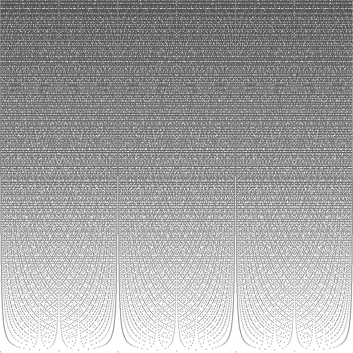
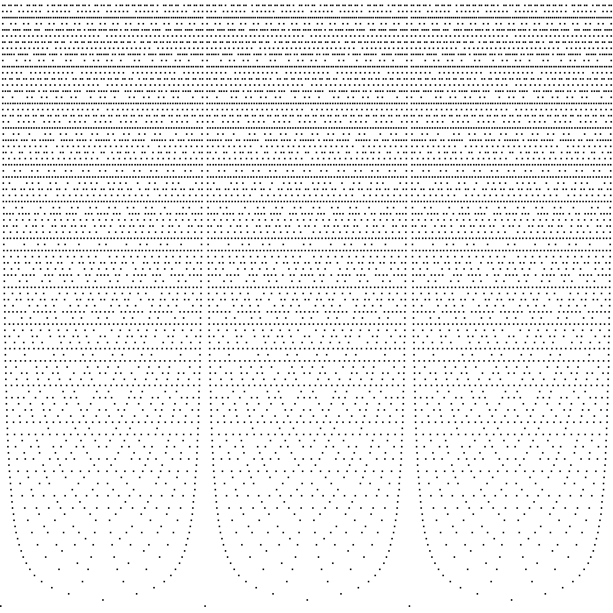
Let us now turn to visualizing rational points in the two sequences $X_1$ and $X_2$. Given a rational point $q$, we will visualize the data pair $(q, h(q))$, where $h$ is a height function. Thus the higher that a point is within the visualization, the higher the height.

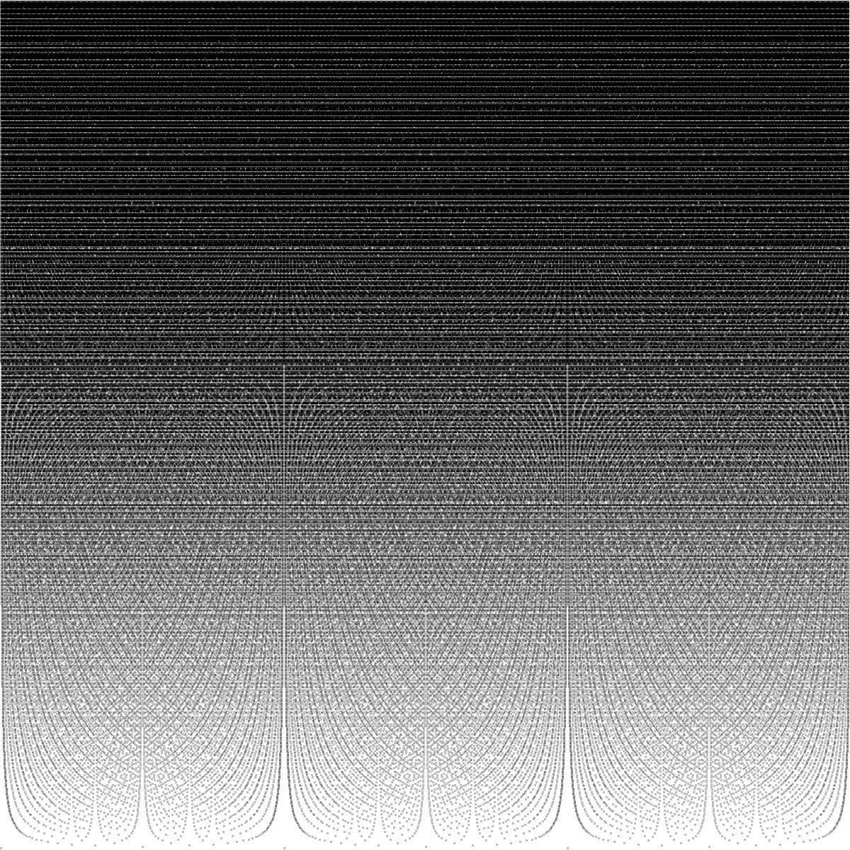
These are images formed from all rationals on $[0, 3]$ with denominator bounded by $400$ (first image) and $100$ (second image). Each point corresponds to a point $(q, h_1(q))$.

These are images formed from all rationals $q$ on $[0, 3]$ with $h_2(q)^2 \leq 70000$ (first image) and $20000$ (second image). Each point corresponds to a point $(q, h_2(q))$.

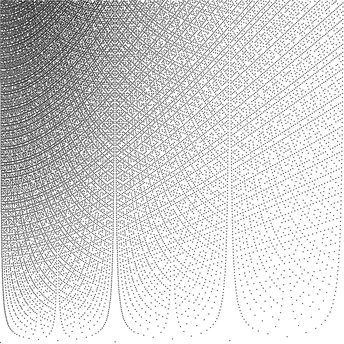
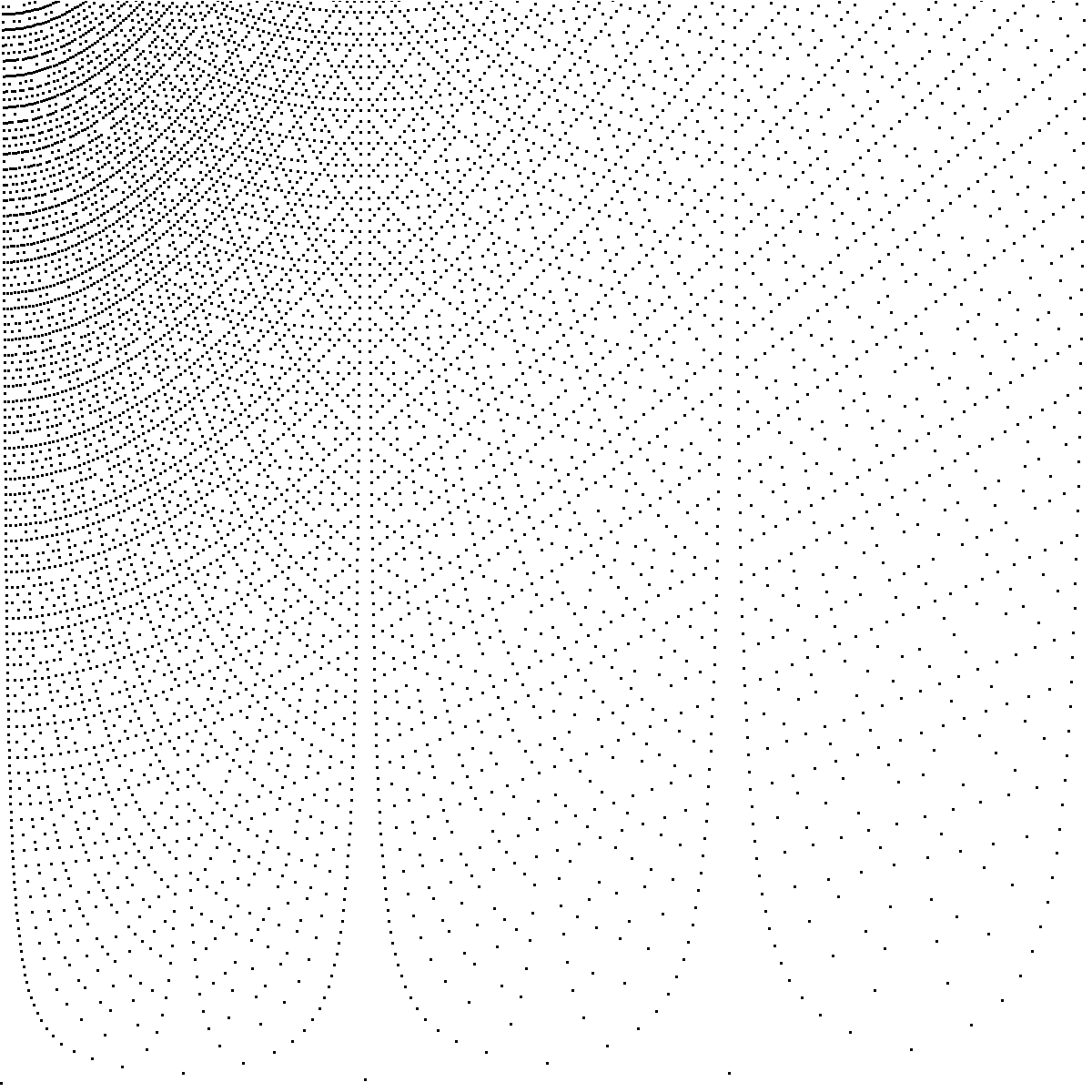
Several patterns emerge from the images. At the bottom of each graph, there are wells in which no points occur. If you examine these wells, you can see that at the bottom center of each well, there is a single rational point. These notably occur around points of low height — most notably around $0, 1/2, 1, 3/2, 2, 5/2, 3$. The reason is simple: for a rational $q = a/b$ to be near $1/2$ (say), we need $1/2 - a/b \sim 1/2b$ to be small, and thus $b$ to be large. In both $h_1$ and $h_2$, the height grows linearly in the denominator $b$. On the other hand, there will be many other pairs of points of similarly bounded height that are much closer. For example, $1/b$ and $1/(b-1)$ are approximately $1/b^2$ apart, which can be significantly closer.^{1 1}My mathematical sibling Alex Walker first described this heuristic to me.

The graphs of $X_1$ visually become uniform, and appear almost to be mildly textured swaths of grey. We can make this even more pronounced, which we do in the next image. Graphs of $X_2$ show a clearly denser set of points at the left (favoring smaller numerators).

We now make a set of related images. In the images that follow, we extend each line from a point $(q, h(q))$ upwards. The effect is that at any designated height $H$, the horizontal line through $h(q) = H$ will include points whose heights are bounded above by $H$. To indicate the density of lines, we use shades of grey. The darker the line, the more rational points.

For $X1$, we make two images. First we have a full image, consisting of points with $h(q) \leq 400$ and $20$ different shades of grey. Second, we have a sparser image, consisting of points with $h(q) \leq 100$ and $12$ different shades of grey. These are still over the interval $[0, 3]$.

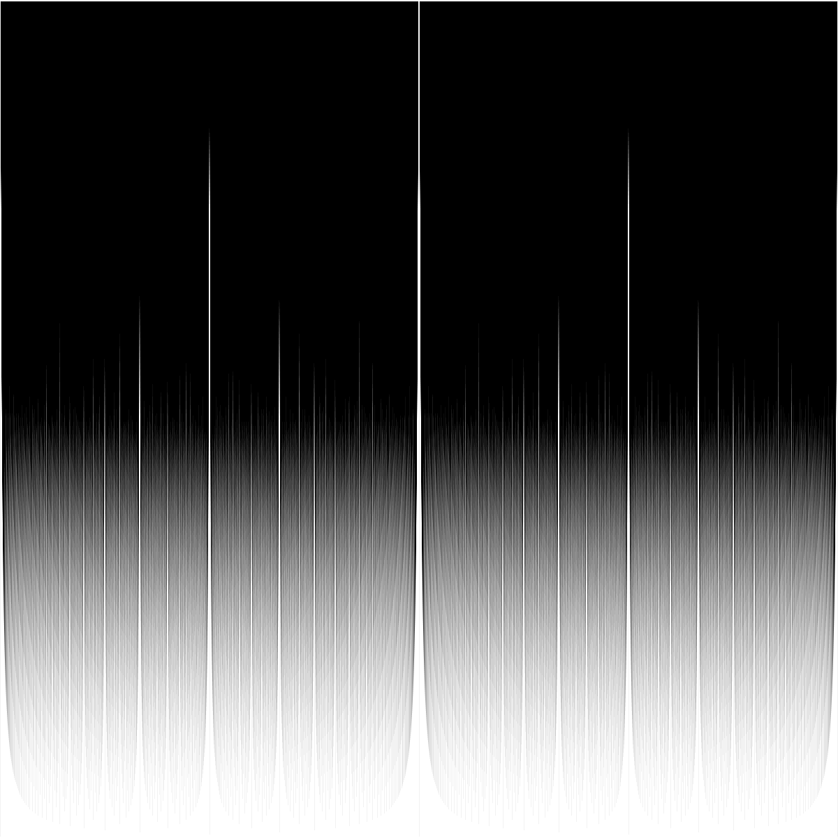
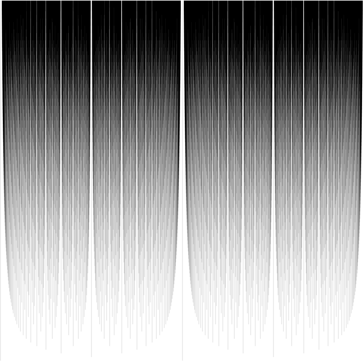
For $X2$, we first have those points with $h(q) \leq 70000$ and $16$ different shades, and then an image with $h(q) \leq 10000$ and $10$ different shades.

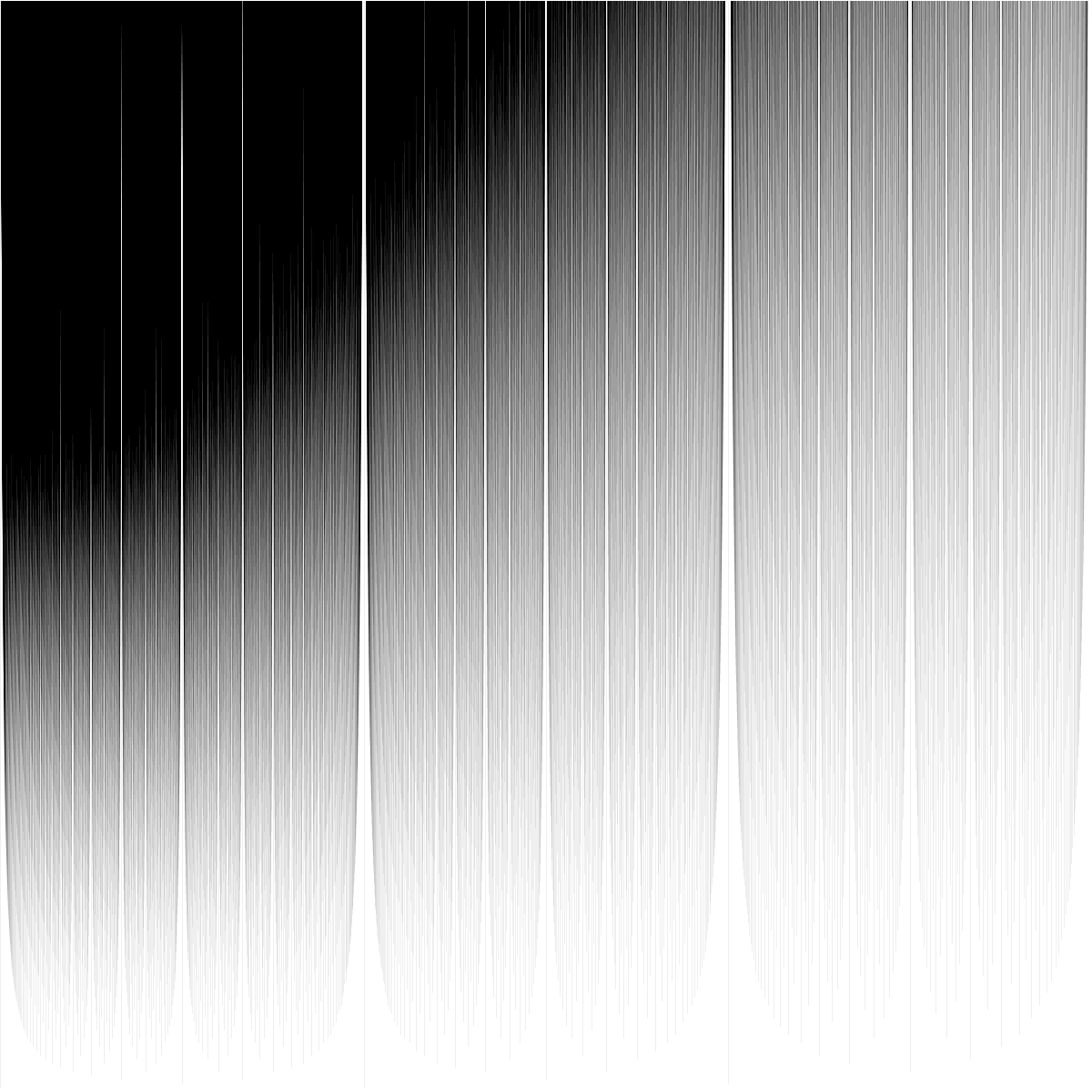
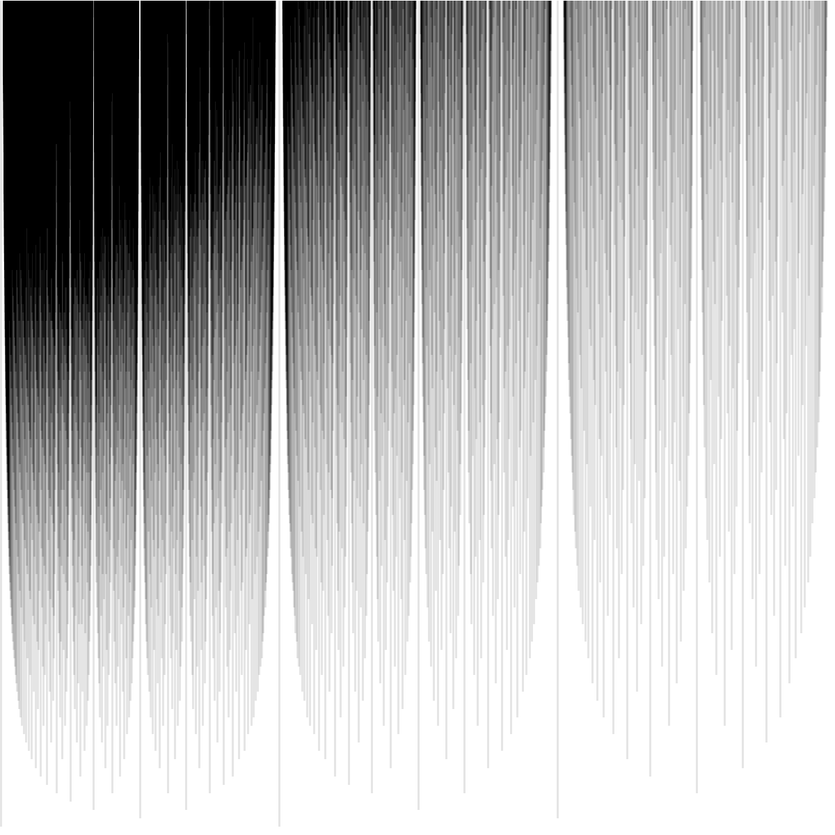
These images really emphasize the wells around rational points of low height. These gives these images their texture.

Leave a comment

Comment via email