MixedMath: Out of Distribution Data, and other experiments for 'ML and vanishing order' Paper

At Harvard's CMSA recent workshop on Math and ML, Alyson Deines and Tamara Deenstra gave a talk that included some of our recent work. (See arxiv link to ML the vanishing order and the reference BBCDLLDOQV25b on my research page.)

To summarize one observation in few words: an $L$-function can be written as

$$ L(s) = \sum_{n \geq 1} \frac{a(n)}{n^s} $$

and satisfies a functional equation of the shape $\Lambda(s) := N^{s} G(s) L(s) = \varepsilon \Lambda(1 - s)$, where $N$ and $\varepsilon$ are distinguished numbers called the conductor and root number, respectively, and where $G(s)$ is a product of gamma factors. We're interested in rational $L$-functions, where the coefficients $a(n)$ are rational numbers when appropriately normalized. These arise from counting questions in number theory and arithmetic geometry.

Conjecturally, the analytic behavior of $L(s)$ at $s = 1/2$ contains deep arithmetic information about the associated counting questions. One such conjecture is the Birch and Swinnerton-Dyer Millenium Conjecture, which says that the order of vanishing at $s = 1/2$ of the $L$-function associated to an elliptic curve agrees with the arithmetic rank of the curve.

No one knows how to prove those results. In BBCDLLDOQV25b, we looked to see if ML might successfully learn something about the order of vanishing from the first several coefficients.

Aside: model success or failure wouldn't say something conclusive about BSD or related conjectures. But in practice, ML can act like a one-sided oracle: if model performance on a particular set of features is very high, this indicates that the arithmetic information is contained within those set of features. If mathematicians don't understand why or how, then at least this can point to a place where we can look for more.

One suggestive graph comes from looking at the 2D PCA. Let's make it here.¹ ¹ This is based on a jupyter notebook. See below for a link to the notebook itself. The data is available at https://zenodo.org/records/14774042. In the code below, this data is in the file lfun_rat_withap.txt.

import pandas as pd
import numpy as np


def is_prime(n):
    "Naive prime detection"
    if n < 2:
        return False
    if n < 4:
        return True
    for d in range(2, int(n**.5) + 2):
        if n % d == 0:
            return False
    return True


assert [p for p in range(20) if is_prime(p)] == [2, 3, 5, 7, 11, 13, 17, 19]


def write_to_float(ap_list):
    """
    Convert the ap string containing aps to a list of ints.
    """
    ap_list = ap_list.replace('[','')
    ap_list = ap_list.replace(']','')
    ap_list = [float(ap) for ap in ap_list.split(',')]
    return ap_list


ALL_COLUMNS = [str(n) for n in range(1,1001)]
PRIME_COLUMNS=[str(p) for p in range(1000) if is_prime(p)]


def write_to_murm_normalized_primes(an_list, w, d = 1):
    """
    Convert the ap strings to a list of normalized floats.
    """
    an_list = an_list.strip('[')
    an_list = an_list.strip(']')
    an_list = [int(an) for an in an_list.split(',')]
    normalized_list = []
    for n, an in enumerate(an_list):
        p=int(PRIME_COLUMNS[n])
        normalization_quotient = d * (p**(w/2.))
        normalized_list.append(np.float32(round(an / normalization_quotient, 5)))
    return normalized_list


def build_murm_ap_df(DF):
    """
    Create a dataframe expanding the single column list of Dirichlet coefficients
    into only prime coefficients, with a single column per prime.
    """
    # Copy all the existing columns except 'ap'
    base = DF.drop(columns=["ap"]).copy()

    # Expand prime coefficients for each row
    prime_expanded = pd.DataFrame(
        [write_to_murm_normalized_primes(a, w, d)
         for w, a, d in zip(DF["motivic_weight"], DF["ap"], DF["degree"])],
        columns=PRIME_COLUMNS,
        index=DF.index
    )
    DF_new = pd.concat([base, prime_expanded], axis=1)
    return DF_new

In the code above, the coefficients are normalized. Coefficient normalization in $L$-functions is an easy source of confusion. Different applicatoins and contexts suggest different obvious normalizations. Instead of detailing this normalization, I'll note that the effect is that the functional equations in this normalization have shape $s \mapsto 1 - s$, and the normalized coefficients vary between $[-1, 1]$.

fname = "lfun_rat_withap.txt"
DF_base = pd.read_table(fname, delimiter=":")

DF_base.head()

	label	primitive	conductor	central character	degree	z1	root analytic conductor	instance types	ap
0	1-1-1.1-r0-0-0	True	1	1.10	1	14.134725	0.004644	['NF', 'DIR', 'Artin', 'Artin']	[1, 1, 1, 1, 1, 1, 1, 1, 1, 1, 1, 1, 1, 1, 1, ...
1	1-5-5.4-r0-0-0	True	5	5.40	1	6.648453	0.023220	['DIR']	[-1, -1, 0, -1, 1, -1, -1, 1, -1, 1, 1, -1, 1,...
2	1-2e3-8.5-r0-0-0	True	8	8.50	1	4.899974	0.037152	['DIR']	[0, -1, -1, 1, -1, -1, 1, -1, 1, -1, 1, -1, 1,...
3	1-12-12.11-r0-0-0	True	12	12.11	1	3.804628	0.055728	['DIR']	[0, 0, -1, -1, 1, 1, -1, -1, 1, -1, -1, 1, -1,...
4	1-13-13.12-r0-0-0	True	13	13.12	1	3.119341	0.060372	['DIR']	[-1, 1, -1, -1, -1, 0, 1, -1, 1, 1, -1, -1, -1...

(Note that you can probably scroll this table if interested).

DF_norm = build_murm_ap_df(DF_base)
DF_norm.head()

	label	primitive	conductor	central character	degree	z1	root analytic conductor	...	937	941	947	953	967	971	977	983	991	997
0	1-1-1.1-r0-0-0	True	1	1.10	1	14.134725	0.004644	...	1.0	1.0	1.0	1.0	1.0	1.0	1.0	1.0	1.0	1.0
1	1-5-5.4-r0-0-0	True	5	5.40	1	6.648453	0.023220	...	-1.0	1.0	-1.0	-1.0	-1.0	1.0	-1.0	-1.0	1.0	-1.0
2	1-2e3-8.5-r0-0-0	True	8	8.50	1	4.899974	0.037152	...	1.0	-1.0	-1.0	1.0	1.0	-1.0	1.0	1.0	1.0	-1.0
3	1-12-12.11-r0-0-0	True	12	12.11	1	3.804628	0.055728	...	1.0	-1.0	1.0	-1.0	-1.0	1.0	-1.0	1.0	-1.0	1.0
4	1-13-13.12-r0-0-0	True	13	13.12	1	3.119341	0.060372	...	1.0	-1.0	-1.0	1.0	-1.0	1.0	-1.0	-1.0	1.0	1.0

5 rows × 179 columns

(Note that you can probably scroll this table if interested).

Now we are ready to do a basic principal component analysis.

from sklearn.decomposition import PCA
from sklearn.preprocessing import StandardScaler

mask = DF_norm["order_of_vanishing"].between(0, 4)
filtered = DF_norm[mask]

X = filtered[PRIME_COLUMNS].values
X = filtered[PRIME_COLUMNS].values
X_scaled = StandardScaler().fit_transform(X)

y = filtered["order_of_vanishing"].values

pca = PCA(n_components=2)
X_pca = pca.fit_transform(X_scaled)

pca_df = pd.DataFrame({
    "PC1": X_pca[:, 0],
    "PC2": X_pca[:, 1],
    "vanishing_order": y
})

This has computed a principal component analysis, and in addition we've populated a small dataframe with data from the two most important components of the PCA. We can plot these components, coloring points based on their vanishing order. One such plot (omitting rank $4$) appears in our paper.

import matplotlib.pyplot as plt


fig, ax = plt.subplots(figsize=[12, 8])
scatter = ax.scatter(
    pca_df["PC1"], pca_df["PC2"],
    c=pca_df["vanishing_order"],
    cmap="viridis",
    alpha=1,
    s=2
)

# Add colorbar and labels
fig.colorbar(scatter, label="vanishing_order")
ax.set_xlabel("Principal Component 1")
ax.set_ylabel("Principal Component 2")
ax.set_title("PCA of PRIME_COLUMNS colored by vanishing_order")
ax.set_xlim(-7.5, 7.5)  # chosen by inspection
ax.set_ylim(-7.5, 7.5)  # not particularly natural

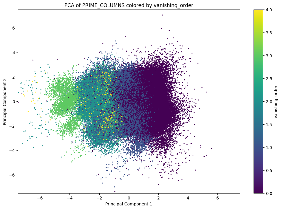
The data for $4$ is so sparse that it's probably a better idea to omit it (and indeed, we omit it in our paper). The point is that these clusters appear to be pretty well-defined, even in only $2$ dimensions. This suggests that linear decision boundaries might suffice to distinguish between vanishing orders. Let's perform a LDA separation.

from sklearn.discriminant_analysis import LinearDiscriminantAnalysis
from sklearn.model_selection import train_test_split
from sklearn.metrics import classification_report, accuracy_score


# Mask rows with vanishing_order between 0 and 4
mask = DF_norm["order_of_vanishing"].between(0, 4)
filtered = DF_norm[mask]

X = filtered[PRIME_COLUMNS].values
y = filtered["order_of_vanishing"].values

# Train/test split
X_train, X_test, y_train, y_test = train_test_split(
    X, y, test_size=0.2, random_state=314159, stratify=y
)

# Scale based only on training data, though I suspect
# it probably doesn't matter in this case.
scaler = StandardScaler()
X_train_scaled = scaler.fit_transform(X_train)
X_test_scaled = scaler.transform(X_test)

lda = LinearDiscriminantAnalysis()
lda.fit(X_train_scaled, y_train)

# Predictions
y_pred = lda.predict(X_test_scaled)

# Evaluate
print("Accuracy:", accuracy_score(y_test, y_pred))
print(classification_report(y_test, y_pred))

Accuracy: 0.8704067775998703
              precision    recall  f1-score   support

           0       0.93      0.84      0.88     22259
           1       0.82      0.90      0.86     19484
           2       0.86      0.92      0.89      6682
           3       0.90      0.77      0.83       742
           4       0.00      0.00      0.00       172

    accuracy                           0.87     49339
   macro avg       0.70      0.69      0.69     49339
weighted avg       0.87      0.87      0.87     49339

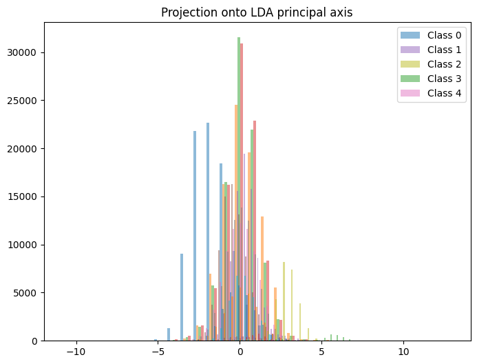
This is consistent with the behavior observed in our paper, and is surprisingly high! It might be interesting to look at the distribution of each rank along the first principal axis. Let's look at histograms to study this distribution.

scores_train = lda.transform(X_train_scaled)
scores_test = lda.transform(X_test_scaled)


fig, ax = plt.subplots(figsize=(8, 6))
# I recognize now that I didn't use the markers, instead I used colors.
# Whoops!
for lab, marker in zip(np.unique(y_train), ['o', 's', '^', 'x', '+']):
    ax.hist(scores_train[y_train==lab], bins=30, alpha=0.5,
            label=f"Class {lab}")
ax.legend()
ax.set_title("Projection onto LDA principal axis")

There is a small cluster of curves with vanishing order $3$ that all have LDA1 just above $5$. I wonder why that is?

As a brief aside, we can ask how much each coefficient matters in this analysis. The coefficients are all normalized to have similar ranges, and thus one could look at the coefficients defining the most import LDA component. A slightly more robust technique is to examine random permutations of the inputs and look at to what extent the predictions deteriorate.

from sklearn.inspection import permutation_importance


r = permutation_importance(lda, X_test_scaled, y_test, n_repeats=50, random_state=314159)
perm_importances = pd.DataFrame({'feature': filtered[PRIME_COLUMNS].columns,
                                 'importance_mean': r.importances_mean,
                                 'importance_std': r.importances_std})
perm_importances.sort_values('importance_mean', ascending=False)

	feature	importance mean	importance std
5	13	0.042678	0.000862
4	11	0.040870	0.000925
3	7	0.040661	0.000815
7	19	0.037700	0.000879
2	5	0.037221	0.000829
...	...	...	...
110	607	0.000384	0.000293
146	853	0.000311	0.000282
153	887	0.000268	0.000240
165	983	0.000192	0.000247
159	941	0.000175	0.000270

168 rows × 3 columns

We have some weak suggestions that the smaller coefficients are more important than later coefficients. We can also look at how much of the variance comes from each component of the LDA.

fig, ax = plt.subplots(figsize=(8, 6))
ax.plot(np.arange(1, len(lda.explained_variance_ratio_)+1),
        lda.explained_variance_ratio_, 'o-')
ax.set_xlabel("Discriminant axis")
ax.set_ylabel("Explained variance ratio")
ax.set_title("Scree plot of LDA discriminant directions")

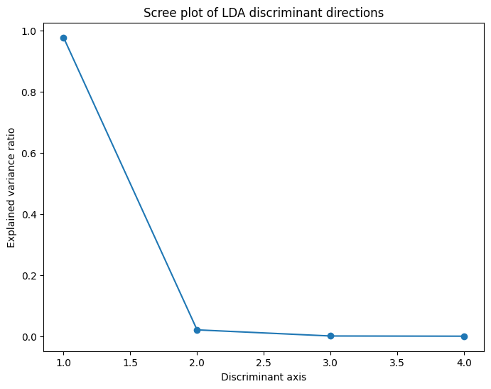
As often happens, the first axis carries the vast majority of the explanatory power.

We can mimic the PCA plot above by plotting the projections onto the first two LDA axes and coloring by order of vanishing. (This plot should look extremely similar, up to some affine transformation due to a lack of canonnical scaling).

X_train_lda = lda.transform(X_train_scaled)
X_test_lda = lda.transform(X_test_scaled)

# Project onto the two most important discriminant axes
fig, ax = plt.subplots(figsize=(8, 6))
for lab in np.unique(y_train):
    ax.scatter(X_train_lda[y_train==lab, 0],
               X_train_lda[y_train==lab, 1],
               alpha=0.6, label=f"Class {lab}", s=2)
ax.set_xlabel("LD1")
ax.set_ylabel("LD2")
ax.legend()
ax.set_title("Multiclass LDA Projection")

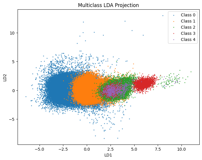
Good, this is very reminiscent of the SVD/PCA analysis plot above.

from sklearn.metrics import confusion_matrix, ConfusionMatrixDisplay

y_pred = lda.predict(X_test_scaled)
cm = confusion_matrix(y_test, y_pred, labels=lda.classes_, normalize='true')
disp = ConfusionMatrixDisplay(confusion_matrix=cm, display_labels=lda.classes_)
disp.plot(cmap='Blues')
ax = disp.ax_
ax.set_title("LDA confusion matrix (test)")

I always like to normalize coloring by true label, so that the darkest blue in a row indicates what predicted label is most common for that true label. This isn't the default normalization.

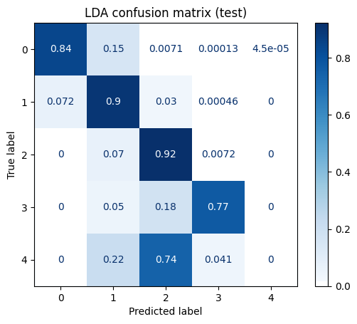
The LDA model identifies orders $0$ to $3$ very well (and completely flails with order $4$, almost certainly due to poor data support).

Out of Distribution Data

Sergei Gukov asked during the talk what happens on out-of-distribution data. Given nonsense, or perhaps misplaced data, what does the model say? Let's see!

Given any set of $168$ real numbers, we can pretend that they are the (normalized) coefficients $a_p$ for primes up to $1000$ of some $L$-function. (Actually, as long as these coefficients are between $-1$ and $1$, they are $\epsilon$-close to some $L$-function).

For example, suppose we choose random integers between $-5$ and $5$, $10$ times, and feed it to our model. What do we get?

# random data
import random

for idx in range(10):
    random_data = np.array([random.randint(-5, 5) for _ in range(168)])
    print(f"v_{idx} prediction: {lda.predict(random_data.reshape(1, -1))[0]}")

v_0 prediction: 3
v_1 prediction: 0
v_2 prediction: 1
v_3 prediction: 2
v_4 prediction: 0
v_5 prediction: 1
v_6 prediction: 0
v_7 prediction: 0
v_8 prediction: 2
v_9 prediction: 0

Let's organize this better.

def uniform_experiment(lower_bound, upper_bound=None, n_iter=10000):
    if upper_bound is None:
        if lower_bound < 0:
            upper_bound = -lower_bound
        else:
            upper_bound = 2 * lower_bound
    random_data = np.random.randint(lower_bound, high=upper_bound, size=(n_iter, 168))
    preds = lda.predict(random_data)
    print(f"After {n_iter} iterations of vectors with entries from "
          f"{lower_bound} to {upper_bound}: avg predicted rank is {preds.mean()}")


for _ in range(10):
    uniform_experiment(-5, 5)

After 10000 iterations of vectors with entries from -5 to 5: avg predicted rank is 2.492
After 10000 iterations of vectors with entries from -5 to 5: avg predicted rank is 2.4833
After 10000 iterations of vectors with entries from -5 to 5: avg predicted rank is 2.4889
After 10000 iterations of vectors with entries from -5 to 5: avg predicted rank is 2.4902
After 10000 iterations of vectors with entries from -5 to 5: avg predicted rank is 2.4959
After 10000 iterations of vectors with entries from -5 to 5: avg predicted rank is 2.5008
After 10000 iterations of vectors with entries from -5 to 5: avg predicted rank is 2.4915
After 10000 iterations of vectors with entries from -5 to 5: avg predicted rank is 2.5016
After 10000 iterations of vectors with entries from -5 to 5: avg predicted rank is 2.4798
After 10000 iterations of vectors with entries from -5 to 5: avg predicted rank is 2.4788

Is it surprising that it's consistent instead of random? I don't know. Let's do a couple of other ranges.

for _ in range(3):
    uniform_experiment(4, 6)
for _ in range(3):
    uniform_experiment(0, 10)
for _ in range(3):
    uniform_experiment(-1, 1)
for _ in range(3):
    uniform_experiment(-10, 0)
for _ in range(3):
    uniform_experiment(-6, -4)

After 10000 iterations of vectors with entries from 4 to 6: avg predicted rank is 0.0
After 10000 iterations of vectors with entries from 4 to 6: avg predicted rank is 0.0
After 10000 iterations of vectors with entries from 4 to 6: avg predicted rank is 0.0
After 10000 iterations of vectors with entries from 0 to 10: avg predicted rank is 0.0
After 10000 iterations of vectors with entries from 0 to 10: avg predicted rank is 0.0
After 10000 iterations of vectors with entries from 0 to 10: avg predicted rank is 0.0
After 10000 iterations of vectors with entries from -1 to 1: avg predicted rank is 2.9779
After 10000 iterations of vectors with entries from -1 to 1: avg predicted rank is 2.9795
After 10000 iterations of vectors with entries from -1 to 1: avg predicted rank is 2.9754
After 10000 iterations of vectors with entries from -10 to 0: avg predicted rank is 3.0
After 10000 iterations of vectors with entries from -10 to 0: avg predicted rank is 3.0
After 10000 iterations of vectors with entries from -10 to 0: avg predicted rank is 3.0
After 10000 iterations of vectors with entries from -6 to -4: avg predicted rank is 3.0
After 10000 iterations of vectors with entries from -6 to -4: avg predicted rank is 3.0
After 10000 iterations of vectors with entries from -6 to -4: avg predicted rank is 3.0

How about from normal distributions?

def gaussian_experiment(center=0, stddev=1, n_iter=10000):
    random_data = np.random.normal(loc=center, scale=stddev, size=(n_iter, 168))
    preds = lda.predict(random_data)
    print(f"After {n_iter} iterations of vectors Gaussian({center}, {stddev}) "
          f"entries: avg predicted rank is {preds.mean()}")


for _ in range(10):
    gaussian_experiment()

After 10000 iterations of vectors Gaussian(0, 1) entries: avg predicted rank is 0.6823
After 10000 iterations of vectors Gaussian(0, 1) entries: avg predicted rank is 0.6896
After 10000 iterations of vectors Gaussian(0, 1) entries: avg predicted rank is 0.6743
After 10000 iterations of vectors Gaussian(0, 1) entries: avg predicted rank is 0.6889
After 10000 iterations of vectors Gaussian(0, 1) entries: avg predicted rank is 0.6911
After 10000 iterations of vectors Gaussian(0, 1) entries: avg predicted rank is 0.6879
After 10000 iterations of vectors Gaussian(0, 1) entries: avg predicted rank is 0.6844
After 10000 iterations of vectors Gaussian(0, 1) entries: avg predicted rank is 0.6937
After 10000 iterations of vectors Gaussian(0, 1) entries: avg predicted rank is 0.6909
After 10000 iterations of vectors Gaussian(0, 1) entries: avg predicted rank is 0.6833

for _ in range(3):
    gaussian_experiment(0, 2)
for _ in range(3):
    gaussian_experiment(-1, 2)
for _ in range(3):
    gaussian_experiment(-1)
for _ in range(3):
    gaussian_experiment(1)
for _ in range(3):
    gaussian_experiment(1, 2)

After 10000 iterations of vectors Gaussian(0, 2) entries: avg predicted rank is 0.8428
After 10000 iterations of vectors Gaussian(0, 2) entries: avg predicted rank is 0.833
After 10000 iterations of vectors Gaussian(0, 2) entries: avg predicted rank is 0.8387
After 10000 iterations of vectors Gaussian(-1, 2) entries: avg predicted rank is 2.9974
After 10000 iterations of vectors Gaussian(-1, 2) entries: avg predicted rank is 2.9983
After 10000 iterations of vectors Gaussian(-1, 2) entries: avg predicted rank is 2.9985
After 10000 iterations of vectors Gaussian(-1, 1) entries: avg predicted rank is 3.0
After 10000 iterations of vectors Gaussian(-1, 1) entries: avg predicted rank is 3.0
After 10000 iterations of vectors Gaussian(-1, 1) entries: avg predicted rank is 3.0
After 10000 iterations of vectors Gaussian(1, 1) entries: avg predicted rank is 0.0
After 10000 iterations of vectors Gaussian(1, 1) entries: avg predicted rank is 0.0
After 10000 iterations of vectors Gaussian(1, 1) entries: avg predicted rank is 0.0
After 10000 iterations of vectors Gaussian(1, 2) entries: avg predicted rank is 0.0
After 10000 iterations of vectors Gaussian(1, 2) entries: avg predicted rank is 0.0
After 10000 iterations of vectors Gaussian(1, 2) entries: avg predicted rank is 0.0

I notice that there is a very strong relationship between having lots of large magnitude, negative coefficients and having large predicted analytic rank. This is very consistent with BSD-type conjectures, which include the conjecture that

$$ \lim_{X \to \infty} \frac{1}{\log X} \sum_{p \leq X} \frac{a_E(p) \log p}{p} = - r + \frac{1}{2}. $$

Thus we should expect a preponderance of early negative coefficients to lead to a larger rank. The LDA has picked up on this broad pattern.

Mestre-Nagao

When first looking at our data, we thought that Mestre-Nagao sums would be closely related. But it wasn't very obvious how. Poking around the various coefficients didn't lead to any obvious connections.

Partially this should be expected. There are random and non-cannonical choices made when performing PCA or LDA separations. In practice, there are indeterminacies up to affine transformations; in cases where there are very similar underlying eigenvalues, components might be transformed to lie anywhere in the subspace spanned by the associated eigenvectors.

What do the eigenvalues look like here?

It is possible to use an eigenvalue solver to produce the LDA in the first place. But I've used the (default, more robust) SVD solver and thus haven't actually computed any eigenvalues explicitly.

Thus here I use a basic implementation that I took from ChatGPT, and which looks write to me.

# Within- and between-class scatter
overall_mean = X_train_scaled.mean(axis=0)
classes = np.unique(y_train)

S_W = np.zeros((X_train_scaled.shape[1], X_train_scaled.shape[1]))
S_B = np.zeros_like(S_W)

for c in classes:
    Xc = X_train_scaled[y_train==c]
    mean_c = Xc.mean(axis=0)
    S_W += np.cov(Xc, rowvar=False) * (Xc.shape[0]-1)
    n_c = Xc.shape[0]
    mean_diff = (mean_c - overall_mean).reshape(-1,1)
    S_B += n_c * (mean_diff @ mean_diff.T)

# Solve generalized eigenproblem
eigvals, eigvecs = np.linalg.eig(np.linalg.pinv(S_W) @ S_B)

# Sort
idx = np.argsort(eigvals)[::-1]
eigvals = eigvals[idx].real
eigvecs = eigvecs[:,idx].real

print("Top eigenvalues (discriminative strength):", eigvals[:5])

Top eigenvalues (discriminative strength): [2.97874807e+00 6.42431948e-02 3.15256533e-03 1.26095142e-03
 2.28691727e-08]

These are pretty different.

This suggests that the method indeterminacy (not coming from fuzzy data, but from the method itself) is mostly limited to affine transformation.

We can use this.² ²I haven't thought of this before, so this is new! If we expect Mestre-Nagao sums to be closely related to the PCA or LDA decomposition, we should try to predict Mestre-Nagao sums affinely from the components.

To be precise, we consider the basic Mestre-Nagao sums

$$ \sum_{p \leq X} \frac{a_p \log p}{p}. $$

There are other closely related sums that are also called Mestre-Nagao, but for the moment let's look at this one. We compare these to projections on the principal LDA axis by "training" an affine model (aka linear regression, the most basic of basic tools) on them.

from sklearn.linear_model import LinearRegression
from sklearn.metrics import r2_score
from sklearn.utils import resample


primes = [p for p in range(1000) if is_prime(p)]
primes = np.array(primes)


def mestre_nagao(X):
    logs = np.log(primes)
    return (X * logs / primes).sum(axis=1)


C_train = mestre_nagao(X_train)
C_test = mestre_nagao(X_test)


X_train_lda = lda.transform(scaler.transform(X_train))  # make sure we have same standardization
ld_cols = [f"LD{i+1}" for i in range(X_train_lda.shape[1])]
lda_df = pd.DataFrame(X_train_lda, columns=ld_cols)
corrs = [np.corrcoef(C_train, X_train_lda[:,k])[0,1] for k in range(X_train_lda.shape[1])]
print("Pearson correlations between C and LD axes (train):")
for k,rval in enumerate(corrs):
    print(f"  LD{k+1}: r = {rval:.4f}")

# Quick scatter of C vs LD1
fig, ax = plt.subplots(figsize=(8,6))
ax.scatter(X_train_lda[:,0], C_train, alpha=0.4, s=4)
ax.set_xlabel("LD1")
ax.set_ylabel("MN(x)")
ax.set_title("Mestre-Nagao vs LD1")

Pearson correlations between C and LD axes (train):
  LD1: r = -0.9589   <– <("<) Wow, what a huge number
  LD2: r = -0.2654
  LD3: r = -0.0488
  LD4: r = 0.0159

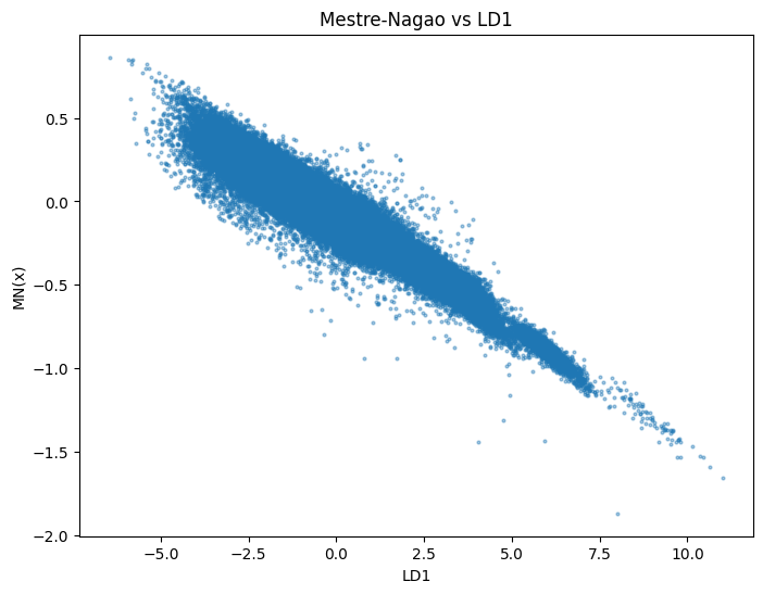
For each (normalized) $L$-function, this plot compares the projection of the data vector associated to that $L$-function on the principal LDA axis against the associated (normalized) Mestre-Nagao sum. And the point seems to be that they are strongly linear correlated! Will you look at that. The Mestre-Nagao sums correlate really obviously with the first discriminant axis.

lr = LinearRegression()
lr.fit(C_train.reshape(-1,1), X_train_lda[:,0])  # just use principal axis
pred = lr.predict(C_train.reshape(-1,1))
r2 = r2_score(X_train_lda[:,0], pred)
print(f"R^2 of regressing LD1 on C (train): {r2:.4f}")

# Let's also look at what happens on the validation data
X_test_lda = lda.transform(scaler.transform(X_test))
pred_test = lr.predict(C_test.reshape(-1,1))
r2_test = r2_score(X_test_lda[:,0], pred_test)
print(f"R^2 on test set: {r2_test:.4f}")

R^2 of regressing LD1 on C (train): 0.9194
R^2 on test set: 0.9201

As a small experiment, what if we add in Mestre-Nagao sums and retrain our predictor. Do we do better?

sc2 = StandardScaler()
X_train_scaled = scaler.transform(X_train)
X_test_scaled  = scaler.transform(X_test)

C_train_scaled = (C_train - C_train.mean()) / (C_train.std(ddof=0) + 1e-12)
C_test_scaled  = (C_test - C_train.mean()) / (C_train.std(ddof=0) + 1e-12)

X_train_aug = np.hstack([X_train_scaled, C_train_scaled.reshape(-1,1)])
X_test_aug = np.hstack([X_test_scaled, C_test_scaled.reshape(-1,1)])

lda_aug = LinearDiscriminantAnalysis()
lda_aug.fit(X_train_aug, y_train)

print("Original LDA train acc:", lda.score(X_train_scaled, y_train), "test acc:", lda.score(X_test_scaled, y_test))
print("Augmented LDA train acc:", lda_aug.score(X_train_aug, y_train), "test acc:", lda_aug.score(X_test_aug, y_test))

print("Explained variance ratio (original):", lda.explained_variance_ratio_)
print("Explained variance ratio (augmented):", lda_aug.explained_variance_ratio_)

Original LDA train acc: 0.8684495880499001 test acc: 0.8704067775998703
Augmented LDA train acc: 0.8684597221236965 test acc: 0.8704067775998703
Explained variance ratio (original): [9.7747040e-01 2.1081256e-02 1.0345095e-03 4.1377844e-04]
Explained variance ratio (augmented): [9.77470147e-01 2.10814738e-02 1.03461600e-03 4.13763677e-04]

There is no additional explanatory power from incorporating Mestre-Nagao sums! That's also interesting, as it suggests that the LDA has gleaned everything it can already.

This suggests more work to do!

Implementation Notes

I wrote this in a jupyter notebook and converted it for display here using nbconvert and my typical blog engine. I also make the jupyter notebook directly available.

I have edited the notebook for content, commentary, style, and presentation for this post. I note again that the underlying data for this notebook is also separately available.

Info on how to comment

To make a comment, please send an email using the button below. Your email address won't be shared (unless you include it in the body of your comment). If you don't want your real name to be used next to your comment, please specify the name you would like to use. If you want your name to link to a particular url, include that as well.

bold, italics, and plain text are allowed in comments. A reasonable subset of markdown is supported, including lists, links, and fenced code blocks. In addition, math can be formatted using $(inline math)$ or $$(your display equation)$$.

Please use plaintext email when commenting. See Plaintext Email and Comments on this site for more. Note also that comments are expected to be open, considerate, and respectful.

Comment via email

mixedmath

Out of Distribution Data

Mestre-Nagao

Implementation Notes

Leave a comment