mixedmath

Suppose we have an elliptic curve $E$ over $\mathbb{Q}$ of conductor $N$. How many coefficients $a_p(E)$ does it take to uniquely identify the isogeny class of $E$? (Two elliptic curves over $\mathbb{Q}$ are isogenous if and only if they have the same $L$-function, so we cannot hope to distinguish isogenous elliptic curves by individual point counts).

This question is at the heart of the paper BCCHLLDNP25, part of a collaboration with Babei, Charton, Costa, Huang, Lee, Narayanan, and Pozdnyakov. In this paper we see if ML models can learn to predict later coefficients from collections of earlier coefficients. Successful predictions would indicate that there is enough structure in early coefficients to uniquely specify later coefficients — and therefore that the initial sets of coefficients uniquely specify the curve.

It would be desirable to directly try to test the classification problem of how many coefficients determine a curve, but it's challenging to formulate a concrete, testable experiment for this. (We return to this in the LMFDB Experiment section below).

Instead we test the presumably harder problem of reconstructing later coefficients from earlier coefficients. This is (probably) a much harder problem!

Extending lists of coefficients

How could one go about recognizing or reconstructing a curve from initial sets of coefficients?

Naive Approach

Suppose we are given $a_2, a_3, \ldots, a_p$ for some number of primes $p$. Equivalently, we are given the number of rational points for some curve $E$ over several finite fields $\mathbb{F}_p$.

How hard is it to directly find a curve with these points?

One approach is to consider it one prime at a time and then to combine the local results together with an application of the Chinese Remainder Theorem.^{1 1}This is like Schoof's algorithm, but in reverse. For example, guess random curves $Y^2 = X^3 + aX + b$ for random $a$ and $b$ in $\mathbb{F}_p$.^{2 2}I'm assuming implicitly here that we look at the short Weierstrass model. Thus one shouldn't look at $\mathbb{F}_2$ or $\mathbb{F}_3$ here.

Sturm's Bound

Concretely, we know that the first $\asymp N$ coefficients will uniquely determine (an isogeny class of) an elliptic curve of conductor $N$ because of the modularity theorem. There is a corresponding modular form of level $N$, and Sturm's bound shows that the first $\asymp N$ coefficients determine the form.

Thus given $\asymp N$ coefficients, one could then construct the entire space of weight $2$, level $N$ modular forms and pluck out the matching one. (This is also computationally demanding).

Approximate Functional Equation

The $L$-function of $E$ will satisfy a functional equation of the shape \begin{equation*} \Lambda(s) := N^{s/2} \Gamma_{\mathbb{C}}(s) L(s) = \pm \Lambda(2 - s), \end{equation*} implying an approximate functional equation that implies morally \begin{equation} \Lambda(s) \approx \sum_{n \geq 1} \frac{a_n(E)}{n^s} V_s(n/\sqrt{N}) \end{equation} for a weight function $V_s(y)$ that decays rapidly when $y > 1$. Stated differently, $\Lambda(s)$ is approximately completely determined by the first $\sqrt{N}$ coefficients. (There is a dual sum of the same length that I omit).

In principle, the coefficients can be retrieved from the analytic behavior of the $L$-function. In practice, this is possibly easier by using a variety of weight functions $V_s$ and combining them in clever ways — Farmer, Koutsoliotas, and Lemurell do this with harder approximate functional equations and less-well behaved objects in their paper on maass forms on GL3 and GL4, for instance.

I don't know of any implementation for the purpose of extending coefficient lists (though this would also be interesting and attainable!), but it is performable in principle. Thus the first $O(\sqrt{N})$ coefficients specify the form and "are enough" to reconstruct later coefficients.

Conjectural Results

If the Riemann Hypothesis is true for Artin $L$-functions, then we actually expect that the first $O(\log^2(N))$ coefficients are enough to uniquely specify the isogeny class. (See Bucur and Kedlaya's An application of the effective Sato-Tate conjecture, Corollary 4.8 for more on this).

This says nothing about how to use these to compute the remaining coefficients.

LMFDB Experiment

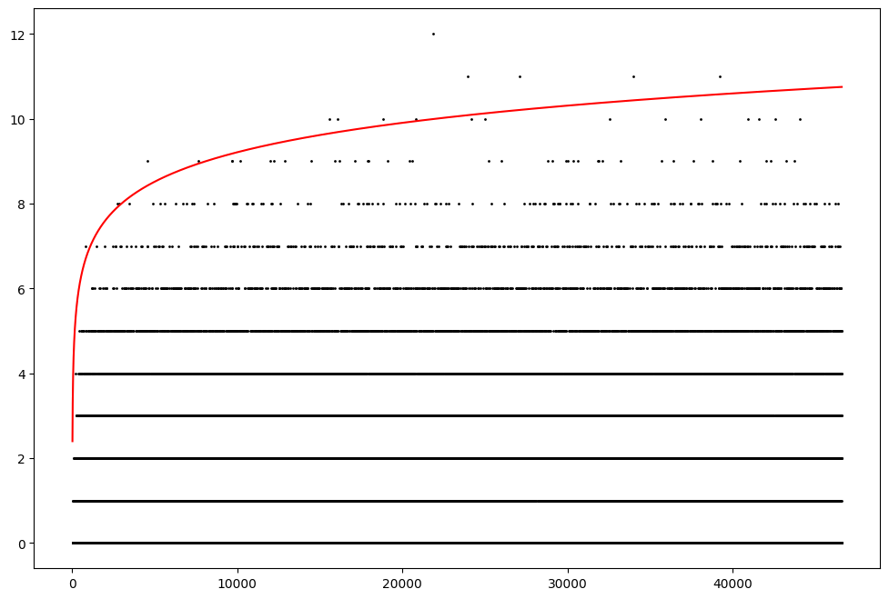
Let's look at the LMFDB's elliptic curves over $\mathbb{Q}$ up to conductor $500{,}000$ (where the table is complete). For every conductor $N$, we compute $B = B(N)$ such that if $E_1$ and $E_2$ are two elliptic curves of conductor $N$, then there exists some $p \leq B$ such that $a_p(E_1) \neq a_p(E_2)$.

Stated differently, we compute the number of $a_p$ coefficients are sufficient to distinguish among all the isogeny classes of elliptic curves of that conductor.

This is a very short data analysis problem with the database available.

# This line is made up, but is approximately right.
# (If you need help accessing LMFDB data, send me
#  or the LMFDB an email and we can help.)
from lmfdb import elliptic_curve_db

def identify_smallest(apcol, conductor, record):
    """
    -1 means unable to distinguish
    0 means only one isogeny class
    otherwise, return B
    """
    m = -1
    if len(apcol) == 1:
        record[conductor] = 0
        return
    for i in range(len(apcol)):
        for j in range(i + 1, len(apcol)):
            found = False
            for idx, (a, b) in enumerate(zip(apcol[i], apcol[j])):
                if a != b:
                    m = max(m, idx)
                    found = True
                    break
            if not found:
                record[conductor] = -1
                return
    record[conductor] = m

record = dict()
cur_conductor = 11
apcol = []
cursor = elliptic_curve_db.search(sort=['conductor'])

while True:
    ec = next(cursor)
    conductor = ec['conductor']
    if conductor != cur_conductor:
        identify_smallest(apcol, cur_conductor, record)
        cur_conductor = conductor
        apcol = []
    apcol.append(ec['aplist'])

Let's plot $B(N)$ and a reasonable curve. Below, I plot $B(N)$ and the curve $\log(N)$.

Looking a bit closer at the smaller range:

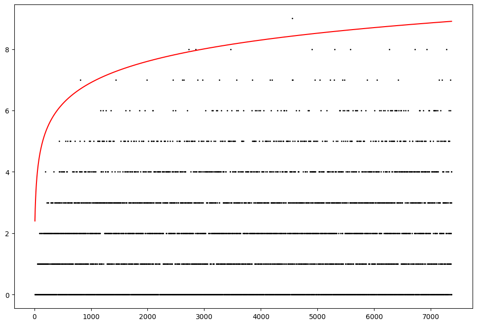
Maybe $\log(N)$ is about right?

Here is one heuristic explanation: we should expect $a_p(E)$ to be semi-circle-random between $-2 \sqrt{p}$ and $2 \sqrt{p}$. Assuming independence for simplicity, specifying $a_p(E)$ thus cuts out a region of density $1/4\sqrt{p}$ from the overall distribution.

There are $\ll N$ isogeny classes of elliptic curves of conductor $N$ (by modularity, these all correspond to a weight $2$ modular form of level $N$. The valence formula there gives the dimension of the space to be $\ll N$).

Heuristically, asking how many $a_p$ it takes to uniquely specify an isogeny class reduces to asking when \begin{equation*} \prod_{p \leq x} \frac{1}{4 \sqrt{p}} \asymp N. \end{equation*} Primorial asymptotics show this occurs approximately when $x \asymp \log N$. Thus maybe we should expect $\log(N)$ to be enough.

Related Notes

These bounds are closely related to the Sturm Bound, Trace Bound, and Distinguishing $T_p$ bound for classical modular forms. (These are links to LMFDB knowls).

In particular, we look at Hecke kernels, distinguishing sets of Hecke operators $T_p$ acting on Galois orbits of newforms. The size of these kernels is often very small, perhaps much smaller than one might expect. On the other hand, the kernels in the LMFDB are constructed greedily in terms of the size of the prime, but the largest prime is sometimes larger than the Sturm bound.

This is to say: it's not quite the same... but it's closely related.

Leave a comment

Comment via email