mixedmath

This is a note written for my fall 2013 Math 100 class, but it was not written "for the exam,'' nor does anything on here subtly hint at anything on any exam. But I hope that this will be helpful for anyone who wants to get a basic understanding of Taylor series. What I want to do is try to get some sort of intuitive grasp on Taylor series as approximations of functions. By intuitive, I mean intuitive to those with a good grasp of functions, the basics of a first semester of calculus (derivatives, integrals, the mean value theorem, and the fundamental theorem of calculus) - so it's a mathematical intuition. In this way, this post is a sort of follow-up of my earlier note, An Intuitive Introduction to Calculus.

We care about Taylor series because they allow us to approximate other functions in predictable ways. Sometimes, these approximations can be made to be very, very, very accurate without requiring too much computing power. You might have heard that computers/calculators routinely use Taylor series to calculate things like ${e^x}$ (which is more or less often true). But up to this point in most students' mathematical development, most mathematics has been clean and perfect; everything has been exact algorithms yielding exact answers for years and years. This is simply not the way of the world.

Here's a fundamental fact to both mathematics and life: almost anything worth doing is probably pretty hard and pretty messy.

For a very recognizable example, let's think about finding zeroes of polynomials. Finding roots of linear polynomials is very easy. If we see ${5 + x = 0}$, we see that ${-5}$ is the zero. Similarly, finding roots of quadratic polynomials is very easy, and many of us have memorized the quadratic formula to this end. Thus ${ax^2 + bx + c = 0}$ has solutions ${x = \frac{-b \pm \sqrt{b^2 - 4ac}}{2a}}$. These are both nice, algorithmic, and exact. But I will guess that the vast majority of those who read this have never seen a "cubic polynomial formula'' for finding roots of cubic polynomials (although it does exist, it is horrendously messy - look up Cardano's formula). There is even an algorithmic way of finding the roots of quartic polynomials. But here's something amazing: there is no general method for finding the exact roots of 5th degree polynomials (or higher degree).

I don't mean We haven't found it yet, but there may be one, or even You'll have to use one of these myriad ways - I mean it has been shown that there is no general method of finding exact roots of degree 5 or higher polynomials. But we certainly can approximate them arbitrarily well. So even something as simple as finding roots of polynomials, which we've been doing since we were in middle school, gets incredibly and unbelievably complicated.

So before we hop into Taylor series directly, I want to get into the mindset of approximating functions with other functions.

1. Approximating functions with other functions

We like working with polynomials because they're so easy to calculate and manipulate. So sometimes we try to approximate complicated functions with polynomials, a problem sometimes called "polynomial interpolation''.

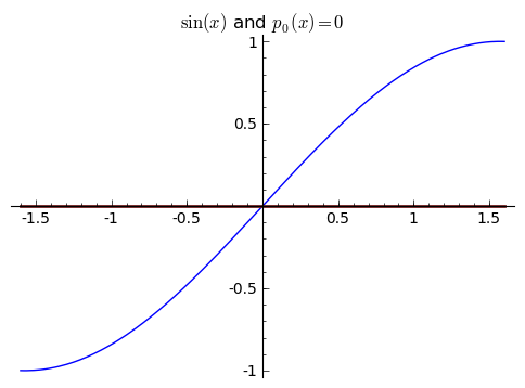
Suppose we wanted to approximate ${\sin(x)}$. The most naive approximation that we might do is see that ${\sin(0) = 0}$, so we might approximate ${\sin(x)}$ by ${p_0(x) = 0}$. We know that it's right at least once, and since ${\sin(x)}$ is periodic, it's going to be right many times. I write ${p_0}$ to indicate that this is a degree ${0}$ polynomial, that is, a constant polynomial. Clearly though, this is a terrible approximation, and we can do better.

1.1. Linear approximation

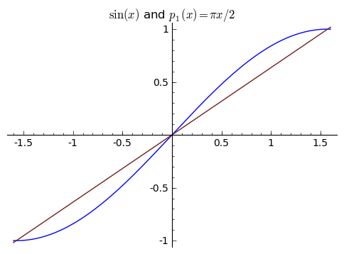
So instead of a constant function, let's approximate it with a line. We know that ${\sin(0) = 0}$ and ${\sin(\pi/2) = 1}$, and two points determine a line. What is the line that goes through ${(0,0)}$ and ${(\frac{\pi}{2}, 1)}$?. It's ${p_1(x) = \frac{2}{\pi}x}$, and so this is one possible degree ${1}$ approximation:

$\displaystyle p_1(x) = \frac{2}{\pi}x. $

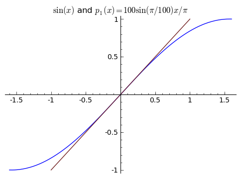
You might see that our line depends on what two points we use, and this is very true. Intuitively, you would expect that if we chose our points very close together, you would get an approximation that is very accurate near those two points. If we used ${0}$ and ${\pi/100}$ instead, we get this picture:

Two points determine a line. I've said this a few times. Alternately, a point on the line and the slope of the line are enough to determine the line. What if we used that ${\sin(0) = 0}$ to give us the point ${(0,0)}$, and used that ${\sin'(0) = \cos(0) = 1}$ to give us our direction? Then we would have a line that goes through the point ${(0,0)}$ and has the right slope, at least at the point ${(0,0)}$ - this is a pretty good approximate. I'll call this line ${T_1(x)}$, and in this case we see that ${T_1(x) = 0 + 1x = x}$. Aside: Some people call the derivative the "best linear approximator'' because of how accurate this approximation is for ${x}$ near ${0}$ (as seen in the picture below). In fact, the derivative actually is the "best'' in thise sense - you can't do better.

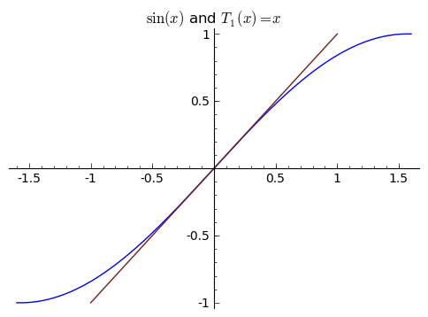
These two graphs look almost the same! In fact, they are very nearly the same, and this isn't a fluke. If you think about it, the secant line going through ${(0,0)}$ and ${(\frac{\pi}{100}, \sin(\pi/100))}$ is an approximation of the derivative of ${\sin(x)}$ at ${0}$ - so of course they are very similar!

1.2. Parabolic approximation

But again, we could do better. Three points determine a parabola. Let's try to use ${\sin(0) = 0}$, ${\sin(\pi/2) = 1}$ and ${\sin(\pi) = 0}$ to come up with a parabola. One way we could do this would be to use that we know both roots of the parabola, ${0}$ and ${\pi}$. So our degree ${2}$ approximation must be of the form ${p_2(x) = a(x-0)(x-\pi)}$, since all degree ${2}$ polynomials with zeroes at ${0}$ and ${\pi}$ are of this form (I am implicitly using something called the Factor Theorem here, which says that a polynomial ${p(x)}$ has a root ${r}$ if and only if ${p(x) = (x-r)q(x)}$ for some other polynomial ${q(x)}$ of degree one less than ${p}$). What is ${a}$? We want it to pass through the point ${(\pi/2, 1)}$, so we want ${p_2(\pi/2) = 1}$. This leads us to ${a(\pi/2)(-\pi/2) = 1}$, so that ${a = -\frac{4}{\pi^2}}$. And so

$\displaystyle p_2(x) = -\frac{4}{\pi^2}x(x-\pi). $

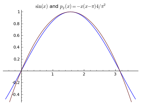
As we can see, the picture looks like a reasonable approximation for ${x}$ near ${\pi/2}$, but as we get farther away from ${\pi/2}$, it gets worse.

Earlier, we managed to determine a line with either 2 points, or a point and a slope. Intuitively, this is because lines look like ${bx + a}$, so there are two unknowns. Thus it takes ${2}$ pieces of information to figure out the line, be they points or a point and a direction. So for a parabola ${cx^2 + bx + a}$, it takes three pieces of information. We've done it for three points. We can also do it for a point, a slope, and a concavity, or rather a point, the derivative at that point, and the second derivative at that point.

Let's follow this idea to find another quadratic approximate, which I'll denote by ${T_2}$ in parallel to my notation above, for ${x}$ around ${\pi/2}$. We'll want ${T_2(\pi/2) = 1}$, ${T'_2(\pi/2)= 0}$, and ${T{}'{}'_2(\pi/2) = -1}$, since ${\sin(\pi/2) = 1, \sin'(\pi/2) = \cos(\pi/2) = 0,}$ and ${\sin{}'{}'(\pi/2) = -\sin(\pi/2) = -1}$. How do we find such a polynomial? The "long'' way would be to call it ${cx^2 + bx + a}$ and create the system of linear equations

$\begin{align*} T_2(\pi/2) &= a(\pi/2)^2 + b(\pi/2) + c\\ T_2'(\pi/2) &= 2a(\pi/2) + b\\ T_2{}'{}'(\pi/2) &= 2a = -1 \end{align*}$

and to solve them. We immediately see that ${a = -\frac12}$, which lets us see that ${b = \frac{\pi}{2}}$, which lets us see that ${c = 1 - \frac{\pi^2}{8}}$. This yields

$\displaystyle T_2(x) = -\frac{1}{2}x^2 + \frac{\pi}{2}x + 1 - \frac{\pi^2}{8}. $

The "clever'' way is to write the polynomial in the form ${T_2(x) = c(x-(\pi/2))^2 + b(x - (\pi/2)) + a}$, since then ${T_2(\pi/2) = a}$ (as the other terms have a factor of ${(x-(\pi/2))}$). When you differentiate ${T_2(x)}$ in this form, you get ${2c(x-(\pi/2)) + b}$, so that ${T_2'(\pi/2) = b}$. And when you differentiate again, you get ${2c}$, so that ${\frac{1}{2}T_2{}'{}'(\pi/2) = c}$. This has the advantange of allowing us to simply read off the answer without worrying about solving the system of linear equations. Putting these together gives

$\displaystyle T_2(x) = -\frac{1}{2}(x-(\pi/2))^2 + 0 + 1. $

And if you check (you should!), you see that these two forms of ${T_2(x)}$ are equal. This feels very "mathlike'' to me. These approximations look like

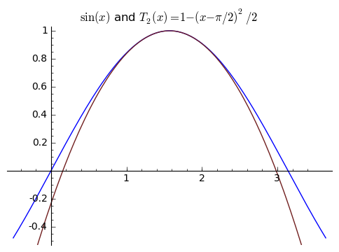
Comparing the two is insteresting. ${p_2}$ is okay near ${\pi/2}$, then gets a bit worse, but then gets a little better again near ${0}$ and ${\pi}$. But ${T_2}$ is extremely good near ${\pi/2}$, and then gets worse and worse.

1.3. Cubic approximation

You can see that ${T_2}$ gives us a better approximation than ${p_2}$ for ${x}$ close to ${\pi/2}$, just as ${T_1}$ was better than ${p_1}$ for ${x}$ near ${0}$. Let's do one more: cubic polynomials. Let's use the points ${-\pi/3, -\pi/6, \pi/6,}$ and ${\pi/3}$ to generate ${p_3}$. This yields

$\begin{align*} p_3 &= \frac{\sin(\frac{-\pi}{3})(x + \frac{\pi}{6})(x - \frac{\pi}{6})(x - \frac{\pi}{3})}{(\frac{-\pi}{3} + \frac{\pi}{6})(\frac{-\pi}{3} - \frac{\pi}{6})(\frac{-\pi}{3} - \frac{\pi}{3})} + \frac{\sin(\frac{-\pi}{6})(x + \frac{\pi}{3})(x - \frac{\pi}{6})(x - \frac{\pi}{3})}{(\frac{-\pi}{6} + \frac{\pi}{3})(\frac{-\pi}{6} - \frac{\pi}{6})(\frac{-\pi}{6} - \frac{\pi}{3})} +\\ &\phantom{=} + \frac{\sin(\frac{\pi}{6})(x + \frac{\pi}{3})(x + \frac{\pi}{6})(x - \frac{\pi}{3})}{(\frac{\pi}{6} + \frac{\pi}{3})(\frac{\pi}{6} + \frac{\pi}{6})(\frac{\pi}{6} - \frac{\pi}{3})} + \frac{\sin(\frac{\pi}{3})(x + \frac{\pi}{3})(x + \frac{\pi}{6})(x - \frac{\pi}{6})}{(\frac{\pi}{3} + \frac{\pi}{3})(\frac{\pi}{3} + \frac{\pi}{6})(\frac{\pi}{3} - \frac{\pi}{6})} \end{align*}$

Showing this calculation is true leads us a bit further afield, but we'll jump right in. Four points, so if we wanted to we could create a system of linear equations as we did above for ${T_2}$ and solve. It may even be a good refresher on solving systems of linear equations. But that's not how we are going to approach this problem today. Instead, we're going to be a bit "clever'' again.

Here's the plan: find a polynomial-part that takes the right value at ${-\pi/3}$ and is ${0}$ at ${-\pi/6, \pi/6}$ and ${\pi/3}$. Do the same for the other three points. Add these together. This is reasonable since it's easy to find a cubic that's ${0}$ at the points ${-\pi/6, \pi/6}$ and ${\pi/3}$: it's ${a(x+\pi/6)(x - \pi/6)(x-\pi/3)}$. We want to choose the value of ${a}$ so that this piece is ${\sin(-\pi/3) = -\sqrt3/2}$ when ${x=-\pi/3}$. This leads us to choosing

$\displaystyle a = \frac{-\sqrt3/2}{(-\pi/3 + \pi/6)(-\pi/3 - \pi/6)(-\pi/3 - \pi/3)}. $

In other words, this polynomial part is

$\displaystyle -\sqrt3/2 \cdot \frac{(x+\pi/6)(x - \pi/6)(x-\pi/3)}{(-\pi/3 + \pi/6)(-\pi/3 - \pi/6)(-\pi/3 - \pi/3)}. $

Written in this form, it's easy to see that it is ${0}$ at the three points where we want it to be ${0}$, and it takes the right value at ${-\pi/3}$. Notice how similar this was in feel to our work for the quadratic part. Doing the same sort of thing for the other three points and adding all four together yields a cubic polynomial (since all four subparts are cubic) that takes the correct values at 4 points. Since there is only 1 cubic that goes through those four points (since four points determine a cubic), we have found it. Aside: this is just a few steps away from being a full note about Lagrange polynomial interpolation. This looks like

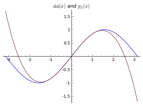
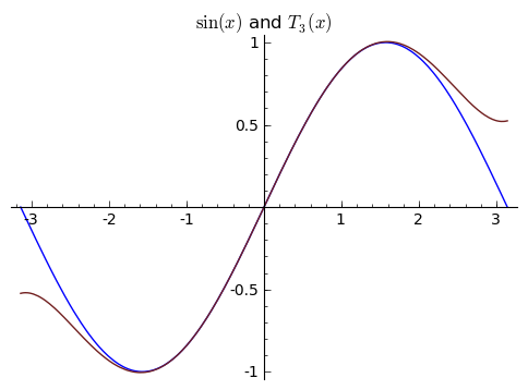
These points were chosen symmetrically around ${0}$ so that this might be a reasonable approximation when ${x}$ is close to ${0}$. How will ${p_3}$ compare to ${T_3}$, the approximating polynomial determined by ${\sin(x)}$ and his derivatives at ${0}$? Our four pieces of information now will be ${\sin(0) = 0, \sin'(0) = \cos(0) = 1, \sin{}'{}'(0) = -\sin(0) = 0,}$ and ${\sin{}'{}'{}'(0) = -\cos(0) = -1}$. Writing ${T_3}$ first as ${T_3(x) = dx^3 + cx^2 + bx + a}$, we see that ${T_2(0) = a}$, ${T'_3(0) = b, T{}'{}'{}_3(0) = 2c,}$ and ${T{}'{}'{}'_3(0) = 3!d}$. This lets us read off the coefficients: we have ${a = 0, b = 1, c = 0, d = -1/6}$, so that in total

$\displaystyle T_3(x) = -\frac{1}{6}x^3 + x, $

which looks like

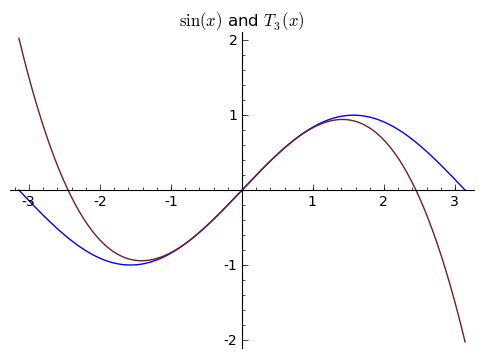
These look very similar. Which one is better? Let's compare the differences between ${p_3(x)}$ and ${\sin(x)}$ with the differences between ${T_3(x)}$ and ${\sin(x)}$ in graph form. This next picture shows ${\sin(x) - p_3(x)}$, or rather the error in the approximation of ${\sin(x)}$ by ${p_3(x)}$. What we want is for this graph to be ${0}$, since this means that ${\sin(x)}$ is exactly ${p_3(x)}$, or as close to ${0}$ as possible. Since the approximation is so good, the picture is very zoomed in.

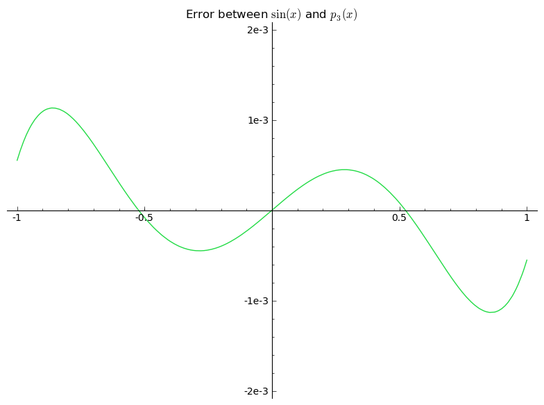
Notice that the y-axis is labelled by "1e-3'', which means ${10^{-3} = .001}$. So the error is within ${0.001}$, which is very small (we really zoomed in). As you can see, the error is a bit weird. It oscillates a little, and is a bit hard to predict. Now let's look at the picture of ${\sin(x) - T_3(x)}$.

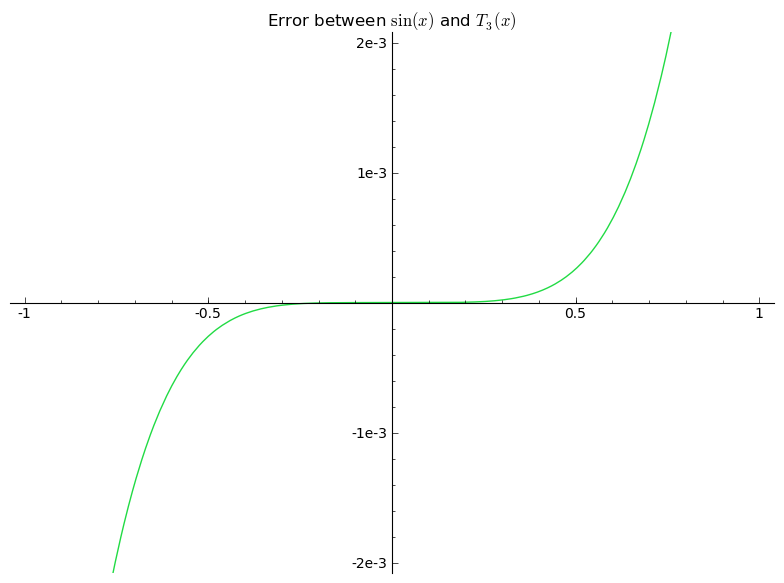
This error is very easy to predict, and again we can see that it is extremely accurate near the point we used to generate the approximation (which is ${0}$ in this case). As we get further away, it gets worse, but it is far more accurate and more predictably accurate in the center. Further, ${T_3(x)}$ was easier to generate than ${p_3(x)}$, and it gives four decimal places of accuracy near ${0}$ while ${p_3(x)}$ can only give two. So maybe there is something special to these ${T}$ polynomials. Let's look into them more.

Aside: people spend a lot of time on these interpolating problems. If this is something you are interested in, let me know and I can direct you to further avenues of learning about them

2. Taylor Polynomials

The idea that the ${T_n(x)}$ polynomials were better approximates than ${p_n(x)}$ around the central point, as we saw above, led to the ${T}$ polynomials getting a special name: they are called "Taylor Polynomials.'' This might not be how you've seen Taylor polynomials introduced before, but this is where they really come from. And this is what keeps the right intuition. Just as the first derivative is the "best linear approximation,'' these Taylor Polynomials give the best quadratic approximation, cubic approximation, etc. Let's get the next few Taylor polynomials for ${\sin(x)}$ for ${x}$ near ${0}$.

We saw that ${T_3(x) = x - \frac{1}{6}x^3}$. And the way we got this was by calculating ${\sin(x)}$ and its first three derivatives at ${0}$ (giving us 4 pieces of information), and finding the unique cubic polynomial satisfying those four pieces of information. So to get more accuracy, we might try to include more derivatives. So let's use the ${\sin(x)}$ and its first four derivatives at ${0}$. These are ${\sin(0) = 0, \sin'(0) = \cos(0) = 1, \sin{}'{}'(0) = -\sin(0) = 0, \sin'{}'{}'(0) = -\cos(0) = -1}$, and ${\sin^{(4)}(0) = \sin(0) = 0}$. Writing ${T_4(x) = ax^4 + bx^3 + cx^2 + dx + e}$, we expect ${T_4(0) = e, T_4{}'(0) = d, T_4{}'{}'(0) = 2c, T_4{}'{}'{}'(0) = 3!b, T^{(4)}_4(0) = 4! a}$. Since the fourth derivative is ${0}$, we get the same polynomial as before! We get ${x - \frac{1}{6}x^3}$. But before we go on, notice that the constant term ${e}$ came from evaluating ${\sin(0)}$, the coefficient of ${x}$ came from evaluating ${\cos(0)}$, the coefficient of ${x^2}$ came from ${\frac{1}{2}\cdot -\sin(0)}$, the coefficient of ${x^3}$ came from ${\frac{1}{3!} \cdot - \cos(0)}$, and the coefficient of ${x^4}$ came from ${\frac{1}{4!} \sin(0)}$. These are exactly the same expressions that came up for ${a,b,c,}$ and ${d}$ from before.

This is something very convenient. We see that the coefficient of ${x^n}$ in our ${T}$ polynomials depends only of the ${n}$th derivative of ${\sin(x)}$. So to find ${T_5}$, I don't need to recalculate all the coefficients. I just need to realize that the coefficient of ${x^5}$ will come from the fifth derivative of ${\sin(x)}$ at ${0}$ (which happens to be ${1}$). And to get this, we would have differentiated ${T_5(x)}$ five times, giving us an extra ${5!}$, so that the coefficient is ${\frac{1}{5!}\cdot \sin^{(5)}(0) = \frac{1}{5!}}$. All told, this means that

$\displaystyle T_5(x) = x - \frac{1}{3!}x^3 + \frac{1}{5!}x^5, $

and that this is the best degree ${5}$ approximation around the point ${0}$. Pictorally, we see

Now that we've seen the pattern, we can write the general degree ${n}$ Taylor polynomial ,${T_n}$, approximation for ${\sin(x)}$:

$\displaystyle T_n(x) = x - \frac{1}{3!}x^3 + \frac{1}{5!}x^5 - \frac{1}{7!}x^7 + \ldots + \frac{1}{n!}\sin^{(n)}(0) = \sum_{k = 0}^{n/2} \frac{(-1)^{k}}{(2k+1)!}x^{2k+1} $

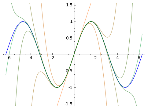
The next images shows increasingly higher order Taylor approximations to ${\sin(x)}$. Worse approximations are more orange, better are closer to blue.

What we've done so far extends very generally. The degree ${n}$ polynomial that agrees with the value and first ${n}$ derivatives of a function ${f(x)}$ at ${x = 0}$ approximates the function ${f(x)}$ for values of ${x}$ near ${0}$, and in general these polynomials are given by

$\displaystyle T_n(x) = \sum_{k = 0}^n \frac{f^{(k)}(0)}{k!} x^k. $

This prompts two big questions. First: how good are these approximations? And second, since using more derivatives gives us better approximations, does using "all'' the derivatives give us the whole function? Rather, if ${f}$ is infinitely differentiable, is it true that ${f(x) = \sum_{k = 0}^n \frac{f^{(k)}(0)}{k!} x^k}$? Or is it at least true that this gives us the "best'' approximation we can get from a single point?

These are big questions, and they are all inter-related. The first question leads to considering the remainder, or error, of Taylor polynomials. And the second leads us to consider infinite Taylor series associated to a function.

3. Estimating the Error of Taylor Polynomial Approximations

If we want to know how well we can expect Taylor polynomials to approximate their associated function, then we need to understand the error, or differences, between the two. We might hope that Taylor polynomials always give very good approximations, or that if we use enough terms, then we can get whatever accuracy we want.

But this is not true.

One good example is the function:

$\displaystyle b(x) = \begin{cases} e^{\frac{-1}{1 - x^2}} & 0 \leq x < 1 \\ 0 & x \geq 1 \end{cases} $

This is often called the bump function, because it looks like

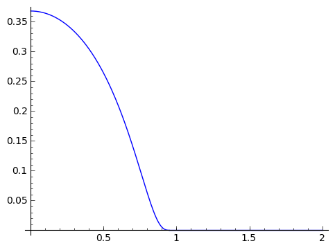
which is just a little bump. The weird thing about this is that ${b(x)}$ is differentiable everywhere. This isn't obvious, because we defined it in two pieces. But it turns out that this function has a derivative even at ${1}$, where the two "pieces'' touch. In fact, this function is infinitely differentiable everywhere. So that's already sort of weird. It's weirder, though, in that all the derivatives of ${b(x)}$ at ${1}$ are exactly ${0}$ (so that these derivatives are more like the derivatives of the constant ${0}$ function to its right than the "bump'' part to its left).

So if you look at the Taylor polynomials for ${b(x)}$ generated at the point ${1}$, then you would get ${T_n(x) = 0}$ for all ${n}$ (all the derivatives are ${0}$). These Taylor polynomials do a terrible job of approximating the bump function.

It turns out that there are many, many functions that are very "nice'' in that they have many derivatives, but which don't have well behaved Taylor approximations. There are even functions that have many derivatives, but whose Taylor polynomials never provide good approximations, regardless of what point you choose to generate the polynomials.

To make good use of Taylor polynomial approximations, we therefore have to be a bit careful about the error in the approximations. To do this, we will use the mean value theorem. (Aside: For those keeping score, the mean value theorem gives us so much. In my previous note, I talk about how the mean value theorem gives us the fundamental theorem of calculus. Now we'll see that it gives us Taylor series and their remainder too. This is sort of crazy, since the statement of the mean value theorem is so underwhelming.)

This also marks a turning point in this note. Suddenly, things become much less experimental and visual. We will prove things - but don't be afraid!

The mean value theorem says that if a function ${f}$ is differentiable, and we choose any two numbers in the domain ${a}$ and ${b}$, then there is a point ${c}$ between ${a}$ and ${b}$ so that ${f'(c)}$ is equal to the slope of the secant line from ${(a, f(a))}$ to ${(b, f(b))}$. Stated differently, there is a point ${c}$ between ${a}$ and ${b}$ so that ${f'(c) = \frac{f(b) - f(a)}{b - a}}$.

If we suppose that ${b = x}$ and ${a = 0}$ (or you could keep ${a}$ as it is for Taylor polynomials generated at points other than ${0}$), then we get that there is some ${c}$ between ${0}$ and ${x}$ such that ${f'(c) = \frac{f(x) - f(0)}{x}}$. Rearranging yields ${f(x) = f(0) + f'(c)x}$. This serves as a bound on the error of the ${0}$ degree Taylor polynomial at ${0}$, which is just ${T_0(x) = f(0)}$. How so? This says that the difference between ${f(x)}$ and ${f(0)}$ (which is our approximate in this case) is at most ${f'(c) x}$ for some ${c}$. If we happen to know that ${f'(c) < M}$ for all ${c}$ in ${[0,x]}$, then we know that ${f(x) - f(0) < Mx}$. So our error at the point ${x}$ is at most ${Mx}$.

This really isn't very good, but it is also a very bad approximate. On the other hand, this semi-trivial example contains the intuition for the proof.

To get a bound on linear approximations, we start off with the derivative of ${f}$. If we apply the mean value theorem of ${f'(x)}$, we get that there is some ${c}$ between ${0}$ and ${x}$ so that ${f{}'{}'(c) = \frac{f'(x) - f'(0)}{x}}$, or rather that ${f'(x) = f'(0) + f''(c)x}$. (This shouldn't be a surprise - ${f'(x)}$ is just a function too, so we expect to get this in the same form as we had above). Here's where we can do something interesting: let's integrate this. In particular, let's rewrite this in ${t}$:

$\displaystyle f'(t) = f'(0) + f''(c)t, $

and let's integrate her:

$\displaystyle \int_0^x f'(t) \mathrm{d}t = \int_0^x f'(0) + f''(c)t \mathrm{d}t. \ \ \ \ \ (1)$

The second fundamental theorem of calculus (which is also essentially the mean value theorem!) says that ${\displaystyle \int_0^x f'(t) \mathrm{d}t = f(x) - f(0)}$. So the equation above becomes

$\displaystyle f(x) - f(0) = xf'(0) + \int_0^xf''(c)t dt. $

How should we think about the second integral? There is a major subtlety here, which is that $c$ depends on each value of $t$ in a difficult-to-predict way. For "nice" functions, we might hope that we can treat $c$ as a constant depending in some way on the entire interval of integration from $0$ to $x$.^{1 1}It is possible to prove that this can be done rigorously, but we will save that for another day. If we treat it as a constant, our expression rearranges to

$\displaystyle f(x) = f(0) + xf'(0) + f''(c)\frac{x^2}{2}. $

This says that the error in our linear Taylor polynomial ${T_1(x) = f(0) + x f'(0)}$ is at most ${f''(c) \frac{x^2}{2}}$ for some ${c}$ in ${[0,x]}$. So as before, if we know a bound ${M}$ on the second derivative, then our error is at most ${Mx^2/2}$. This is much better than what we had above. In particular, if our ${x}$ value is close to ${0}$, like say less than ${1/10}$, then the ${x^2}$ bit in the error means the error has a factor of ${1/100}$. But as we get further away from ${0}$, we expect worse error. This is why in the pictures above we see that the Taylor polynomials give very good approximations near the center of the expansion, and then get predictably worse.

Let's do one more, to see how this works. Now we will start with the second derivative. The mean value theorem says again that ${f''(x) = f''(0) + f'{}'{}'(c)x}$. Writing this in ${t}$ and integrating both sides (with the same unproven assumptions about $f''(c)$ as above), we get

$\begin{align*} \int_0^x f''(t) \mathrm{d}t &= \int_0^x ( f''(0) + f'{}'{}'(c)t ) \mathrm{d}t\\ f'(x) - f'(0) &= f''(0)x + f'{}'{}'(c)\frac{x^2}{2}. \end{align*}$

Rearranging gives

$\displaystyle f'(x) = f'(0) + f''(0)x + f'{}'{}'(c)\frac{x^2}{2}. $

(This shouldn't surprise us either, since the second derivative is just a function. So of course it has a first order expansion just like we saw above.) Let's again write this in ${t}$ and integrate both sides,

$\begin{align*} \int_0^x f'(t)\mathrm{d}t &= \int_0^x (f'(0) + f''(0)t + f'{}'{}'(c)\frac{t^2}{2}) \mathrm{d}t\\ f(x) - f(0) &= f'(0)x + f''(0)\frac{x^2}{2} + f'{}'{}'(c)\frac{x^3}{3!}. \end{align*}$

Rearranging yields

$\displaystyle f(x) = f(0) + f'(0)x + f''(0)\frac{x^2}{2} + f'{}'{}'(c)\frac{x^3}{3!}, \ \ \ \ \ (2)$

for some ${c}$ between ${0}$ and ${x}$. Now we see that the approximations are getting better. Firstly, for ${x}$ near ${0}$, we now get a cubic factor in the error term. So if we were interested in ${x}$ around ${1/10}$, now the error would get a factor of ${1/1000}$. That's pretty good. We also see that there is a rising factorial in the denominator of the error term. If there is anything to know about factorials, it's that they grow very, very fast. So we might hope that this factorial increases with higher derivatives so that the error is even better. (And this is the case).

So the only possible bad thing in this error term is that ${f'{}'{}'(x)}$ is not well-behaved, or is not very small, or is very hard to understand. And in these cases, the error might be very large. This is the case with the bump function above - the derivatives grow too rapidly.

If you were to continue this process, you would see that the general pattern is

$\displaystyle f(x) = f(0) + f'(0)x + f''(0)\frac{x^2}{2} + \ldots + f^{(n)}(0)\frac{x^n}{n!} + f^{(n+1)}(c)\frac{x^{n+1}}{(n+1)!} \ \ \ \ \ (3)$

for some ${c}$ between ${0}$ and ${x}$. And this is where the commonly quoted Taylor remainder estimate comes from:

$\displaystyle \left|f(x) - T_n(x) = f(x) - \left(f(0) + f'(0)x + \ldots + f^{(n)}(0)\frac{x^n}{n!}\right)\right| \leq M \frac{x^{n+1}}{(n+1)!}, $

where ${M}$ is the maximum value that ${|f^{(n+1)}(c)|}$ takes on the interval ${[0,x]}$.

There are other ways of getting estimates on the error of Taylor polynomials, but this is by far my favorite. Now that we have estimates for the error, how can we put that to good use?

Let's go back to thinking about the Taylor polynomials for ${\sin(x)}$ that was the source of all the pictures above. What can we say about the error of the degree ${n}$ Taylor polynomial for ${\sin(x)}$? We can say a lot! The derivatives of ${\sin(x)}$ go in a circle: ${\sin(x) \mapsto \cos(x) \mapsto -\sin(x) \mapsto -\cos(x) \mapsto \sin(x)}$. And all of these are always bounded below by ${-1}$ and above by ${1}$. So the ${(n+1)}$st derivative of ${\sin(x)}$ is always bounded by ${\pm 1}$. By the remainder we derived above, this means that

$\displaystyle |\sin(x) - T_n(x)| \leq M\frac{x^{n+1}}{(n+1)!}| \leq 1\frac{x^{n+1}}{(n+1)!}. $

For small ${x}$, this converges really, really fast - this is why the successive approximations above were so accurate. But it also happens that as ${n}$ gets bigger, the factorial in the denominator grows very fast too - so we get better and better approximations even for not small ${x}$. This prompts another question: what would happen if we kept on including more and more terms? What could we say then? This brings us to the next topic.

4. Taylor Series

Now we know the ${n}$th Taylor polynomial approximates ${\sin(x)}$ very well, and increasingly well as ${n}$ increases. So what if we considered the limit of the Taylor polynomials? Rather, what if we considered

$\displaystyle \lim_{n \rightarrow \infty} T_n(x) = \sum_{k = 0}^\infty \frac{(-1)^nx^{2k + 1}}{(2k+1)!}. $

This is a portal into much deeper mathematics, and is the path that many of the mathematical giants of the past followed. You see, infinite series are weird. When do they exist? Is an infinite sum of continuous functions still continuous? What about differentiable? These are big, deep questions that are beyond the scope of this note. But some of the intuition is totally within the scope of this note.

We know the error of the ${n}$th Taylor polynomial to ${\sin(x)}$ is bounded above by ${\frac{x^{n+1}}{(n+1)!}}$. If we take the limit as ${n\rightarrow \infty}$ of the sequence of remainders, we get

$\displaystyle \lim_{n \rightarrow \infty} \frac{x^{n+1}}{(n+1)!} \rightarrow 0, $

and it goes to ${0}$ no matter what ${x}$ is. (Factorials grow larger than the numerator for any fixed ${x}$). So no matter what ${x}$ is, as we use more and more terms, the approximations become arbitrarily good. In fact, since the error goes to ${0}$ and is well-behaved, we have a powerful result:

$\displaystyle \sin(x) = \sum_{n = 0}^\infty \frac{(-1)^nx^{2n + 1}}{(2n+1)!}. $

That is equality. Not approximately equal to, but total equality. Some people even go so far as to define ${\sin(x)}$ by that Taylor series. When I say Taylor series, I mean the infinite sum. People study Taylor series to try to see what information they can glean about functions from their Taylor series. For example, we know that ${\sin(x)}$ is periodic. But how would you determine that from its Taylor series? (It's not very easy).

It turns out that you can tell a lot about a function from its Taylor series (although not as much as we might like, and we don't really study this in math 100). Functions that are completely equal to their Taylor series are called "analytic'' functions, and analytic functions are awesome. But even Taylor polynomials are good, and used to approximate hard-to-understand things.

Aside: I do a lot of work with complex numbers (where we allow ${i = \sqrt{-1}}$ and things like that) instead of real numbers. One reason why I prefer complex numbers is that complex analytic functions, which are complex-valued functions that are exactly equal to their Taylor series, are miraculous things. Being complex analytic is totally amazing, and you can tell essentially anything you want from the Taylor series of a complex analytic function. This is to say that you are on the precipice of exciting and very deep mathematics. Of course, that's where introductory classes stop.

5. Conclusion

We saw Taylor polynomials, some approximations, some proofs, and some Taylor series. One thing I would like to mention is that for applications, people normally use finite Taylor polynomials and show (or use, if it's well known) that the error is small enough for the application. But Taylor polynomials are useless without some understanding of the error. In Math 100, we give a totally lackluster treatment of error estimates. Serious math and physics concentrators will probably need and use more than what we have taught - even though now is perhaps the best time to learn it. So it goes! (Others might very well use Taylor polynomials and their error, but many useful functions and their remainders are understood just as well as those for sine, which we saw here; it is not always necessary to reinvent the wheel, although it can be rewarding in less immediate ways).

I hope you made it this far. If you have any comments, questions, concerns, tips, or whatnot then feel free to leave a comment or to ask me. For additional reading, I would advise you to use only google and free materials, as everything is available for free (and I mean legally and freely available). Something I did not mention but that I've been thinking about is presenting a large collection of applications of Taylor series. Perhaps another time.

This note can be found online at mixedmath.wordpress.com or davidlowryduda.com under the title "An Intuitive Overview of Taylor Series.'' This note was written with vim in latex, and converted to html by a modified latex2wp. Thus this document also comes in pdf and .tex code . The pdf does not include my beautiful gif, which I am always proud of. The graphics were all produced using the free mathematical software sage . Interestingly, this note was the source of sage trac 15419, which will likely result in a tiny change in sage as a whole. I highly encourage people to check sage out.

And to my students - I look forward to seeing you in class. We only have a few left.

Leave a comment

Comment via email