This is a post written for my fall 2013 Math 100 class but largely intended for anyone with knowledge of what a function is and a desire to know what calculus is all about. Calculus is made out to be the pinnacle of the high school math curriculum, and correspondingly is thought to be very hard. But the difficulty is bloated, blown out of proportion. In fact, the ideas behind calculus are approachable and even intuitive if thought about in the right way.
Many people managed to stumble across the page before I'd finished all the graphics. I'm sorry, but they're all done now! I was having trouble interpreting how Wordpress was going to handle my gif files - it turns out that they automagically resize them if you don't make them of the correct size, which makes them not display. It took me a bit to realize this. I'd like to mention that this actually started as a 90 minute talk I had with my wife over coffee, so perhaps an alternate title would be "Learning calculus in 2 hours over a cup of coffee."
So read on if you would like to understand what calculus is, or if you're looking for a refresher of the concepts from a first semester in calculus (like for Math 100 students at Brown), or if you're looking for a bird's eye view of AP Calc AB subject material.
1. An intuitive and semicomplete introduction to calculus
We will think of a function $ {f(\cdot)}$ as something that takes an input $ {x}$ and gives out another number, which we'll denote by $ {f(x)}$. We know functions like $ {f(x) = x^2 + 1}$, which means that if I give in a number $ {x}$ then the function returns the number $ {f(x) = x^2 + 1}$. So I put in $ {1}$, I get $ {1^2 + 1 = 2}$, i.e. $ {f(1) = 2}$. Primary and secondary school overly conditions students to think of functions in terms of a formula or equation. The important thing to remember is that a function is really just something that gives an output when given an input, and if the same input is given later then the function spits the same output out.1 1 As an aside, I should mention that the most common problem I've seen in my teaching and tutoring is a fundamental misunderstanding of functions and their graphs.
For a function that takes in and spits out numbers, we can associate a graph. A graph is a two-dimensional representation of our function, where by convention the input is put on the horizontal axis and the output is put on the vertical axis. Each axis is numbered, and in this way we can identify any point in the graph by its coordinates, i.e. its horizontal and vertical position. A graph of a function $ {f(x)}$ includes a point $ {(x,y)}$ if $ {y = f(x)}$.
Thus each point on the graph is really of the form $ {(x, f(x))}$. A large portion of algebra I and II is devoted to being able to draw graphs for a variety of functions. And if you think about it, graphs contain a huge amount of information. Graphing $ {f(x)= x^2 + 1}$ involves drawing an upwards-facing parabola, which really represents an infinite number of points. That's pretty intense, but it's not what I want to focus on here.
1.1. Generalizing slope - introducing the derivative
You might recall the idea of the 'slope' of a line. A line has a constant ratio of how much the $ {y}$ value changes for a specific change in $ {x}$, which we call the slope (people always seem to remember rise over run). In particular, if a line passes through the points $ {(x_1, y_1)}$ and $ {(x_2, y_2)}$, then its slope will be the vertical change $ {y_2 - y_1}$ divided by the horizontal change $ {x_2 - x_1}$, or $ {\dfrac{y_2 - y_1}{x_2 - x_1}}$.
So if the line is given by an equation $ {f(x) = \text{something}}$, then the slope2 2 For those that remember things like the 'standard equation' $ {y = mx + b}$ or 'point-slope' $ {(y - y_0) = m(x - x_0)}$ but who have never thought or been taught where these come from: the claim that lines are the curves of constant slope is saying that for any choice of $ {(x_1, y_1)}$ on the line, we expect $ {\dfrac{y_2 - y_1}{x_2 - x_1} = m}$ a constant, which I denote by $ {m}$ for no particularly good reason other than the fact that some textbook author long ago did such a thing. Since we're allowing ourselves to choose any $ {(x_1, y_1)}$, we might drop the subscripts - since they usually mean a constant - and rearrange our equation to give $ {y_2 - y = m(x_2 - x)}$, which is what has been so unkindly drilled into students' heads as the 'point-slope form.' This is why lines have a point-slope form, and a reason that it comes up so much is that it comes so naturally from the defining characteristic of a line, i.e. constant slope.
from two inputs $ {x_1}$ and $ {x_2}$ is $ {\dfrac{f(x_2) - f(x_1)}{x_2 - x_1}}$.
But one cannot speak of the 'slope' of a parabola.
Intuitively, we look at our parabola $ {x^2 + 1}$ and see that the 'slope,' or an estimate of how much the function $ {f(x)}$ changes with a change in $ {x}$, seems to be changing depending on what $ {x}$ values we choose. (This should make sense - if it didn't change, and had constant slope, then it would be a line). The first major goal of calculus is to come up with an idea of a 'slope' for non-linear functions. I should add that we already know a sort of 'instantaneous rate of change' of a nonlinear function. When we're in a car and we're driving somewhere, we're usually speeding up or slowing down, and our pace isn't usually linear. Yet our speedometer still manages to say how fast we're going, which is an immediate rate of change. So if we had a function $ {p(t)}$ that gave us our position at a time $ {t}$, then the slope would give us our velocity (change in position per change in time) at a moment. So without knowing it, we're familiar with a generalized slope already. Now in our parabola, we don't expect a constant slope, so we want to associate a 'slope' to each input $ {x}$. In other words, we want to be able to understand how rapidly the function $ {f(x)}$ is changing at each $ {x}$, analogous to how the slope $ {m}$ of a line $ {g(x) = mx + b}$ tells us that if we change our input by an amount $ {h}$ then our output value will change by $ {mh}$.
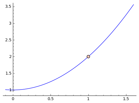
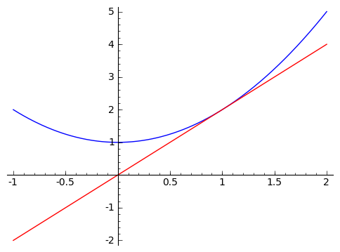
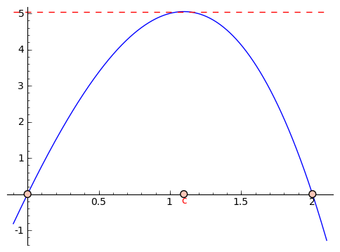
How does calculus do that? The idea is to get closer and closer approximations. Suppose we want to find the 'slope' of our parabola at the point $ {x = 1}$. Let's get an approximate answer. The slope of the line coming from inputs $ {x = 1}$ and $ {x = 2}$ is a (poor) approximation. In particular, since we're working with $ {f(x) = x^2 + 1}$, we have that $ {f(2) = 5}$ and $ {f(1) = 2}$, so that the 'approximate slope' from $ {x = 1}$ and $ {x = 2}$ is $ {\frac{5 - 2}{2 - 1} = 3}$. But looking at the graph,
we see that it feels like this slope is too large. So let's get closer. Suppose we use inputs $ {x = 1}$ and $ {x = 1.5}$. We get that the approximate slope is $ {\frac{3.25 - 2}{1.5 - 1} = 2.5}$. If we were to graph it, this would also feel too large. So we can keep choosing smaller and smaller changes, like using $ {x = 1}$ and $ {x = 1.1}$, or $ {x = 1}$ and $ {x = 1.01}$, and so on. This next graphic contains these approximations, with chosen points getting closer and closer to $ {1}$.
Let's look a little closer at the values we're getting for our slopes when we use $ {1}$ and $ {2, 1.5, 1.1, 1.01, 1.001}$ as our inputs. We get
\begin{equation*} \begin{array}{c|c} \text{second input} & \text{approx. slope} \\ \hline 2 & 3 \\ 1.5 & 2.5 \\ 1.1 & 2.1 \\ 1.01 & 2.01 \\ 1.001 & 2.001 \end{array} \end{equation*}
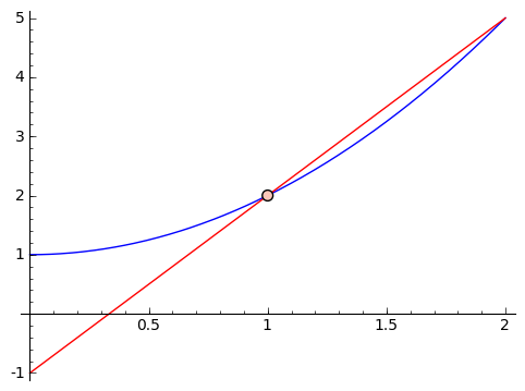
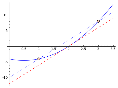
It looks like the approximate slopes are approaching $ {2}$. What if we plot the graph with a line of slope $ {2}$ going through the point $ {(1,2)}$?
It looks great! Let's zoom in a whole lot.
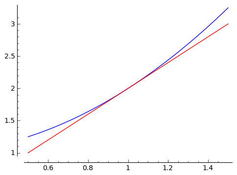
That looks really close! In fact, what I've been allowing as the natural feeling slope, or local rate of change, is really the line tangent to the graph of our function at the point $ {(1, f(1))}$. In a calculus class, you'll spend a bit of time making sense of what it means for the approximate slopes to 'approach' $ {2}$. This is called a 'limit,' and the details are not important to us right now. The important thing is that this let us get an idea of a 'slope' at a point on a parabola. It's not really a slope, because a parabola isn't a line. So we've given it a different name - we call this 'the derivative.' So the derivative of $ {f(x) = x^2 + 1}$ at $ {x = 1}$ is $ {2}$, i.e. right around $ {x = 1}$ we expect a rate of change of $ {2}$, so that we expect $ {f(1 + h) - f(1) \approx 2h}$. If you think about it, we're saying that we can approximate $ {f(x) = x^2 + 1}$ near the point $ {(1, 2)}$ by the line shown in the graph above: this line passes through $ {(1,2)}$ and it's slope is $ {2}$, what we're calling the slope of $ {f(x) = x^2 + 1}$ at $ {x = 1}$.
Let's generalize. We were able to speak of the derivative at one point, but how about other points?
What we did was look at a sequence of points $ {2, 1.5, 1.1, 1.01, 1.001, \dots}$ getting closer and closer to $ {1}$, and finding the slopes of the corresponding lines. So we were calculating $ {\frac{f(2) - f(1)}{2 - 1}}$, $ {\frac{f(1.5) - f(1)}{1.5 - 1}}$, \dots. Seen in a slightly different way, we had a decreasing $ {h}$, starting with $ {1, .5, .1, .01, .001}$ and we were looking at slopes between the inputs $ {x}$ and $ {x + h}$. So we were calculating $ {\frac{f(x + h) - f(x)}{x + h - x} = \frac{f(x+h)-f(x)}{h}}$. We did this for when $ {x = 1}$ and when $ {h = 1, .5, .1, \dots}$ so find the derivative at $ {x = 1}$. But this idea leads to the same process for any $ {x}$. Let's reparse this formula.
$ {\dfrac{f(x+h) - f(x)}{x + h - x} = \dfrac{f(x+h) - f(x)}{h}}$ finds the slope between the points $ {(x,f(x))}$ and $ {(x+h, f(x+h))}$, which approximates the slope at the point $ {x}$. For small $ {h}$, this approximation should be even better. So to find the derivative (read the 'slope') at a value of $ {x}$, we insert that value of $ {x}$ and try this for decreasing $ {h}$. And hopefully it will approach a number, like it approached $ {2}$ above. If this does approach a number like above, then we say that $ {f(x)}$ is differentiable at $ {x}$, and we call the resulting slope the derivative, which we denote by $ {f'(x)}$. So above, when $ {f(x) = x^2 + 1}$, the derivative at $ {x = 1}$ is $ {2}$, or $ {f'(1) = 2}$.
In general, we have
The derivative of a function $ {f(x)}$ at the point $ {x}$, which is an analogy of slope for nonlinear functions, is given by \begin{equation*} f'(x) = \frac{ f(x+h) - f(x) }{h} \tag{1} \end{equation*} as $ {h}$ gets smaller and smaller (if it exists). If this does not tend to some number as $ {h}$ gets smaller and smaller, when $ {f}$ does not have a derivative at $x$. If $ {f}$ has a derivative at $ {x}$, then $ {f}$ is said to be 'differentiable' at $ {x}$.
We haven't really talked about cases when a function doesn't have a derivative, but not every function does. Functions with discontinuities or jumps, or that aren't defined everywhere, etc. don't have good ideas of local slopes. So sometimes functions have derivatives, sometimes they don't, and sometimes they have derivatives at some points and not at others.
Another thing we haven't yet addressed is the notation. Derivatives also have a function-like notation, and that's because they are a function. Above, for $ {f(x) = x^2 + 1}$, we had that $ {f'(1) = 2}$, i.e. the derivative of $ {f}$ at $ {1}$ is $ {2}$. It turns out that $ {f(x) = x^2 + 1}$ has a derivative everywhere (i.e. is called 'differentiable'), and the derivative is given by the function $ {f'(x) = 2x}$. This is an amazingly compact presentation of information. So the 'slope' of $ {f(x) = x^2 + 1}$ at a point $ {x}$ is given by $ {2x}$, for any point $ {x}$. Whoa.
But the important thing to accept now is that we have a way of talking about the 'slope,' or rather the local rate of change, of reasonable-behaving nonlinear functions, and the key is given by Definition 1 above.
1.2. What can we do with a derivative?
A good question now is $ \dots$ so what? Why do we care about derivatives? We mentioned that the derivative gives a good linear approximation to functions (like why our line is so close to the graph of the parabola above). This linear approximation is very useful and important in its own right. We've also mentioned that derivatives give you a way to talk about rates of change, which is also very important in its own right. But I'll mention 3 more things now, and a few in Section$\S$(sec:integrals), when we talk about 'undoing derivatives.'
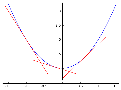
First and most commonly talked about is optimization. Sometimes you want to make something as big, as small, or as cheap as possible. These problems, when you're trying to maximize or minimize something, are called optimization problems. Derivatives provide a method of solving optimization problems (in many ways, the best method). This relies on the key observation that if you have a differentiable (i.e. has a derivative) function $ {f(x)}$ that takes a maximum value when $ {x = c}$, so that $ {f(c) > f(x)}$ for $ {x}$ near $ {c}$, then the 'slope' of $ {f(x)}$ at $ {c}$ will be $ {0}$. In other words, $ {f'(c) = 0}$. Why? Well, this slope describes the slope of the line tangent to $ {f(x)}$ at $ {c}$, and if it's not flat then the function is going up in one direction or the other - and so $ {f(x)}$ isn't a max afterall. An example is shown in the image below:
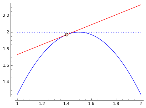
Similarly, if $ {f(x)}$ takes a minimum when $ {x = b}$, then $ {f'(b) = 0}$.
So to maximize or minimize a function, we can calculate its derivative (well, we can't because we're not focusing on the calculations right now, but it's possible and you learn this in a calculus course) and try to find its zeroes. This is really used all the time, and is simple enough to be done automatically. So when companies try to maximize profits, or land use is optimized, or power consumption minimized, etc., there's probably calculus afoot.
Second (although a bit complicated - if you don't understand, don't worry), derivatives give good ways to find zeroes of functions through something called 'Newton's Method.' The idea is that derivatives give linear approximations to our function, and it's easy to see when a line has a zero. So you try to find a point near a zero, approximate the function with a line using a derivative, and find the zero of the line. This will an approximate zero. Repeating this process (approximate the function with a line, find the zero, plug this zero into the function and approximate with a line again) can very quickly yield zeroes. So conceivably you'll be optimizing a function, and thus will find its derivative and want to find its zeroes. So you then use derivatives to find the zeroes of the derivative of the original function\dots in other words, derivatives everywhere.
Third and perhaps most importantly (because this ends up yielding the key to the sections below, because it's not at all obvious how important this is) is a deceptively simple statement. In the first reason above, we talked about how the derivative of a differentiable function at a max or a min is zero. This leads to Rolle's Theorem,
which says that if $ {f(x)}$ is differentiable and $ {f(a) = f(b)}$ for some $ {a}$ and $ {b}$, then there is a $ {c}$ between $ {a}$ and $ {b}$ such that $ {f'(c) = 0}$. The reasoning behind Rolle's Theorem is very simple: if $ {f(a) = f(b)}$ and f is not constant, then there is a max or a min between $ {a}$ and $ {b}$. At this max or min, the derivative is $ {0}$. And if $ {f}$ is constant, then it is a line of slope zero, and thus has derivative $ {0}$.
Using slightly more refined thinking (which amounts to 'rotating a graph' to be level so that we can appeal to Rolle's Theorem), we can get a similar theorem called the Mean Value Theorem:
Suppose $ {f(x)}$ is a differentiable function and $ {a < b}$. Then there is a point $ {c}$ between $ {a}$ and $ {b}$ such that \begin{equation*} \frac{f(b) - f(a)}{b - a} = f'(c).\tag{2} \end{equation*} In other words, there is a point between $ {a}$ and $ {b}$ whose derivative, or immediate slope, is the same as the average slope of $ {f}$ from $ {a}$ to $ {b}$.
Let's use this for a moment to really prove something that sort of know to be true, but that now we can really justify. Let's say that you travel 30 miles in 30 minutes. If we think of your position as a function of time, then we might think of $ {p(0) = 0}$ (so at time $ {0}$, you have gone zero distance) and $ {p(30) = 30}$ (so 30 minutes in, you've gone 30 miles). Your average speed was $ {30}$ miles per $ {30}$ minutes, or $ {60}$ miles per hour. By the mean value theorem, there was at least one time when you were going exactly $ {60}$ miles per hour. If cops were to use this to measure speed, like have strips and/or cameras that record your positions at different times, then they could issue speeding tickets without ever actually measuring your speed. That's sort of cool.
There are many more reasons why derivatives are awesome - but this is what a calculus course is for.
1.3. Undoing derivatives - introducing the integral
So we're done talking about derivatives (mostly). Two big questions motivate the 'other half' of calculus: if I give you the derivative $ {f'(x)}$ of a function, can you 'undifferentiate' it and find the original function $ {f(x)}$? (This is the intrinsic motivation, how you might motivate it yourself from learning derivatives for the first time). But there is also an extrinsic motivation, sort of in the same way that derivatives arise from wanting to talk about slopes of nonlinear functions. This extrinsic motivation is: how do you calculate the area under a function $ {f(x)}$? It's not at all obvious that these are related (real math is full of these surprising and deep connections).
We will proceed with the second one: how do we calculate the area under a function $ {f(x)}$? For this section, we'll start with the function $ {f(x) = 2x}$.
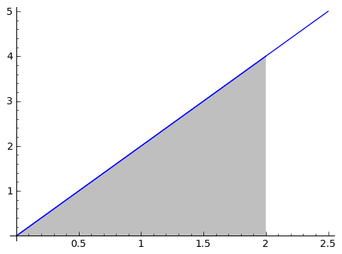
We actually know how to calculate the area under a triangle. Suppose we want to calculate the area between the horizontal axis and $ {f(x)}$, starting at $ {0}$ and going as far right as $ {x}$. So we have a triangle of width $ {x}$ and height $ {2x}$, so the area is $ {\frac{1}{2} x \cdot 2x = x^2}$. Think back to earlier: we found the derivative of $ {x^2 + 1}$ to be $ {2x}$, and now the area from $ {0}$ to $ {x}$ under $ {2x}$ is $ {x^2}$. They almost undid each other! This is an incredible relationship. Let's look deeper.
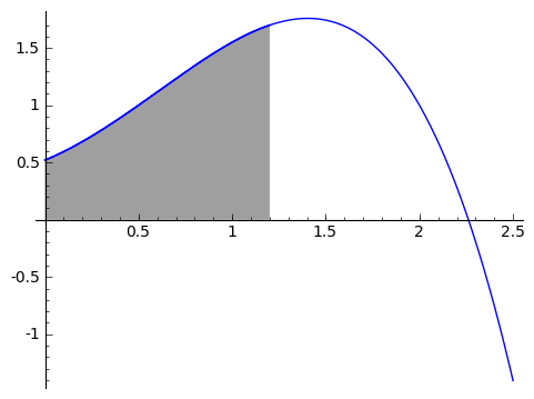
Let's think about a generic well-behaved function $ {f(x)}$, like the picture below.
We're going to create a function called $ {\displaystyle \mathop{Area}_ {(0 \text{ to } x)} (f)},$ which takes in a nice always-positive function $ {f}$ and spits out the area between the function and the horizontal axis from $ {0}$ to $ {x}$. So this is a function in a variable, $ {x}$ - but it's formulated a bit differently (it's right around here where some people may need to adjust how they think of functions). In terms of the function from the graph above, the area represented by $ {\displaystyle \mathop{Area}_ {(0 \text{ to } 1.2)} (f)}$ is the area of the shaded region in the picture below.
Let's do something a bit interesting: let's try to take the derivative of $ {\displaystyle \mathop{Area}_{(0 \text{ to } x)} (f)}$ at $ {x}$. Recall that a derivative of a function $ {f(x)}$ is gotten from looking at $ {\dfrac{f(x+h) - f(x)}{h}}$ as $ {h \rightarrow 0}$. So we want to try to make sense of
\begin{equation*} \frac{\displaystyle \mathop{Area}_{(0 \text{ to } x+h)} (f) - \displaystyle \mathop{Area}_{(0 \text{ to } x)} (f)}{h}.\tag{3} \end{equation*}
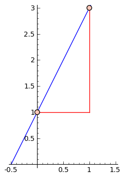
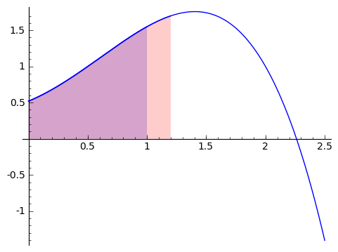
Well, this is finding the area from $ {0}$ to $ {x+h}$ and then taking out the area from $ {0}$ to $ {x}$. If you think about it, we're just left with the area from $ {x}$ to $ {x+h}$, or $ {\displaystyle \mathop{Area}_{(x \text{ to } x+h)} (f)}$. Pictorally, this picture shows the area from $ {0}$ to $ {1}$ in blue, and the area from $ {0}$ to a bit more than $ {1}$ in red (so that the overlap is purple). So in the picture, we are treating $ {x}$ as $ {1}$, so that we're taking the derivative at $ {1}$.
Once we remove the image in blue from the image in red (so we take away everything in purple), we are left with a strip from $ {1}$ to a bit more than $ {1}$, as shown here.
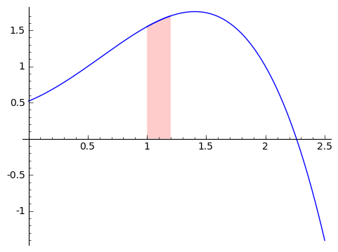
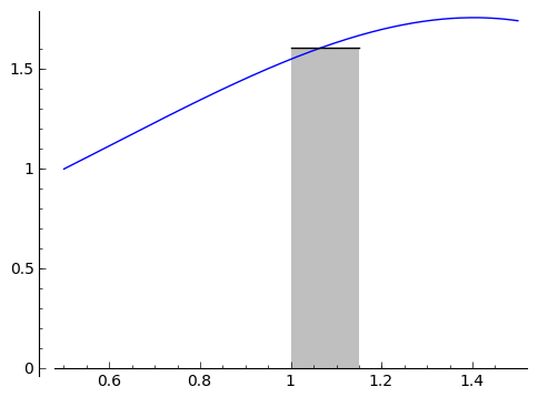
It's time to appeal to a bit of intuition (or the intermediate value theorem ). The area from $ {x}$ to $ {x+h}$ under $ {f}$ is the same as the area of a rectangle of length $ {h}$ and height within the range of $ {f}$ on $ {[x, x+h]}$. For example, the area from the shape above (zoomed in a bit here)
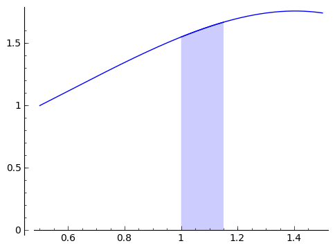
is the same as the area in this rectangle.
Now as $ {h}$ is getting smaller, the height of the rectangle must get closer and closer to $ {f(x)}$, i.e. the value of $ {f}$ at the point $ {x}$. In fact, as $ {h}$ gets smaller, the area from $ {x}$ to $ {x+h}$ under $ {f}$ gets closer and closer to $ {f(x)\cdot h}$ (which is the same as the width of the rectangle times the approximate height), so $ {\displaystyle \mathop{Area}_{(x \text{ to } x+h)} (f) \approx f(x)h}$. This lets us evaluate our derivative:
\begin{equation*} \frac{\displaystyle \mathop{Area}_{(0 \text{ to } x+h)} (f) - \displaystyle \mathop{Area}_{(0 \text{ to } x)} (f)}{h} = \end{equation*} \begin{equation*} = \frac{\displaystyle \mathop{Area}_{(x \text{ to } x+h)} (f)}{h} \approx \frac{f(x)h}{h} = f(x) \end{equation*}
so that taking the derivative of this area function gives back the original function $ {f}$. This is known as the First Fundamental Theorem of Calculus.3 3Aside: remember, this is just an intuitive introduction. There are annoying requirements and assumptions on the functions we're using and ways to make the $ {h \rightarrow 0}$ style arguments rigorous, but I sweep these under the rug for now.
The derivative of the area under a function $ {f}$ from $ {0}$ up to $ {x}$, which we write as $ {\displaystyle \mathop{Area}_{(0 \text{ to } x)} (f)}$, is precisely $ {f(x)}$, the value of the function $ {f}$ at $ {x}$.
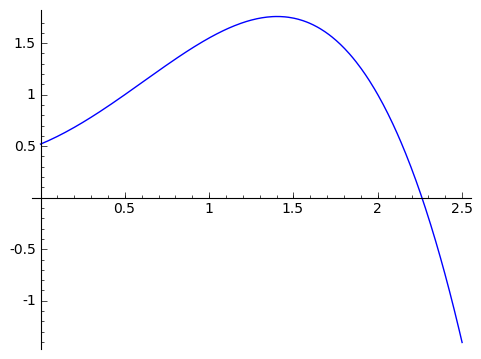
There is a big caveat to what we've just said, and it has to do with this 'Area function.' When does it make sense to talk about the area under a function? For example, what if we have the following function:
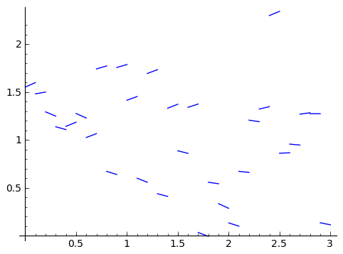
Does it have an area function? What about a worse function, with points all on their own? What do we mean by area? We know how to find areas of polygons and straight-sided shapes. What about non-straight-sided shapes? Just like how we developed derivatives to talk about slopes of nonlinear functions, we will now develop a method to calculate areas of non-straight-sided functions. And just like with derivatives, we're going to do this with approximations.
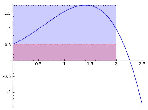
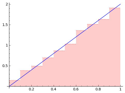
We love being asked to find areas of rectangles, because it's so easy. So given a function and a region on the horizontal axis, say from $ {0}$ to $ {2}$, we can approximate the area by a rectangle. Well, how do we choose how tall to make the rectangle? Let's compare two alternatives: using the minimum value of $ {f}$ on $ {[0,2]}$ (using a minimum-rectangle approximation), and the maximum value of $ {f}$ on $ {[0,2]}$ (using a maximum-rectangle approximation). Let's return to our generic function from above. In blue is the maximum-rectangle approximation, in red in the minimum-rectangle approximation (purple is overlap).
But this is clearly a poor approximation. How can we make it better? What if we used two rectangles? Or three? Or ten? Maybe a hundred?
In the animation above, note that as the number of rectangles increases, the approximation becomes better and better, and our two alternative area methods are getting closer and closer. If, as the number of rectangles gets huge, the area given by the minimum-rectangles tends to the same number $ {A}$ as the area given by the maximum-rectangles, then we say that the area under $ {f}$ from $ {0}$ to $ {2}$ is that number $ {A}$ that the approximations tend to (so this agrees with our intuition in the picture). This is a clear parallel to how we thought of derivatives.
We call the area under a function $ {f(x)}$ from $ {a}$ to $ {b}$ the number $ {A}$ that arises as the number that both the minimum-rectangles approximation and maximum-rectangles approximation tend to as the number of rectangles increases, if there is such a number. If there is such a number, we call $ {f(x)}$ integrable on $ {[a,b]}$, and we represent this area by the symbol \begin{equation*} A = \int_a^b f(t) dt, \tag{4} \end{equation*} where I used $ {t}$ to emphasize that the area is not a function of $ {x}$, but is just the area under a fixed region from $ {a}$ to $ {b}$.
So let's set up the parallel: if we can find the slope of a function at a point (which we call the derivative), we call the function differentiable there; if we can find the area under a function on a region (which we call the integral), we call the function integrable there.
With new notation, we can phrase the first Fundamental Theorem of Calculus as follows: if $ {f}$ is integrable, then the derivative of $ {\displaystyle \int_0^x f(t) dt}$ is $ {f(x)}$. Said another way, we can find functions that can be differentiated to give $ {f(x)}$. For this reason, integrals are sometimes called anti-derivatives. There is a deeper connection here too.
Suppose $ {F(x)}$ is a function whose derivative $ {F'(x)}$ is another function $ {f(x)}$. So $ {F'(x) = f(x)}$. We've seen this relationship so far: the function $ {F(x) = x^2 + 1}$ has derivative $ {f(x) = 2x}$. Let's return to the task of finding the area under $ {f(x)=2x}$, this time from $ {0}$ to $ {1}$. The following is a bit slick and the most non-obvious part of this post (in my opinion/memory).
Start with $ {F(1) - F(0)}$. Let's carve up the segment $ {[0,1]}$ into many little pieces of width $ {0.1}$, i.e. $ {0, 0.1, 0.2, 0.3, \dots, 0.9, 1}$. Then by adding and subtracting $ {F}$ evaluated at these points, we see that
$ \displaystyle F(1) - F(0) = $
$ \displaystyle = (F(1) - F(0.9)) + (F(0.9) - \dots - F(0.1)) + (F(0.1) - F(0)) $
Let's just look at the first set of parentheses for a moment: $ {(F(1) - F(0.9))}$. By the Mean Value Theorem (Theorem 2), we know that
$ \displaystyle \frac{F(1) - F(0.9)}{1 - 0.9} = F'(c_1) = f(c_1) $
for some $ {c_1}$ between $ {.9}$ and $ {1}$, and recalling that $ {F'(x) = f(x)}$. Rearranging this, we get that
$ \displaystyle F(1)- F(0.9) = (1 - 0.9)f(c_1) = 0.1 f(c_1). $
Repeating, we see that
$ \displaystyle F(1) - F(0) = 0.1f(c_1) + 0.1f(c_2) + \ldots + 0.1 f(c_{10}). \ \ \ \ \ (5)$
Here's the magic. This sum has an interpretation. Since $ {c_1}$ is between $ {.9}$ and $ {1}$, and we're multiplying $ {f(c_1)}$ by $ {.1}$, that could be the same calculation we would do if we were approximating the area under $ {f(x)}$ from $ {0}$ to $ {1}$ with $ {10}$ rectangles: each rectangle has width $ {.1}$, so that's why we multiply by $ {.1}$. Then $ {f(c_1)}$ is a reasonable height of the rectangle. So the sum of $ {.1}$ times $ {f(c)}$ values on the right is an approximation of the area under $ {f(x)}$ from $ {0}$ to $ {1}$.
As we use more and more rectangles, it becomes the area, so we get that the area under $ {f(x)}$ from $ {0}$ to $ {1}$ is exactly $ {F(1) - F(0)}$.
Stated more generally (as there was nothing special about $ {[0,1]}$ here):
If $ {F}$ is a differentiable function with $ {F' = f}$, then \begin{equation*} \int_a^b f(t)dt = F(b) - F(a)\tag{6} \end{equation*}
So, for example, to find the area under $ {2x}$ from $ {4}$ to $ {10}$, we can compute $ {F(10) - F(4)}$ where $ {F(x) = x^2 + 1}$, since $ {F'(x) = 2x}$ is the function whose area we want to understand. This gives $ {F(10) - F(4) = 101 - 17 = 84}$. Although $ {2x}$ is not a hard function to compute areas for, this works for many many functions. In fact, integrals are the best tool we have to compute areas when available.
One way of thinking about these big theorems is that the first fundamental theorem says that antiderivatives exist, and the second says that you can use any antiderivative to calculate the area under a function (I haven't mentioned this, but antiderivatives are not unique! $ {F(x) = x^2}$ also has derivative $ {F'(x) = 2x}$, and you can check that it gives the same area under $ {2x}$ from $ {4}$ to $ {10}$). So a large part of calculus is learning how to find antiderivatives for functions you want to study/integrate. What makes this so challenging is that there is no good, general method of finding antiderivatives - so you have to learn a lot of patterns and do a lot of computations. (We don't do any of that here)
This concludes the theoretical development of calculus in AP Calculus AB, and Math 90 at Brown for that matter. But I'd like to mention one under-emphasized fact about the material we've discussed here - this will be the final section.
1.4. Why do we care about integrals, other than to calculate area?
Being able to compute areas is cool and useful in its own right, but I think it's also way over-emphasized. Integrals and derivatives, the two fundamental tools of calculus, allow an entirely different method of thinking about and solving problems. Let's look at two examples.
Population growth
Let's make a model for population growth from first principles. The great strength of calculus is that we can base our calculations only on assumptions of related rates of change. For instance, suppose that $ {P(t)}$ is the population of bacteria in a petri dish at time $ {t}$. We might guess that if there is twice as much bacteria, then there will be twice as much growth (since there will be twice as much bacteria splitting and doing bacteria-reproductive things). Stated in terms of derivatives, we think that the rate of change in bacteria population is proportional to the size of the population, i.e. $ {P'(t) = kP(t)}$ for some constant $ {k}$.
Calculus allows one to 'undo the derivative' on $ {P(t)}$ using integration (and a few things that are not in the scope of this survey), and in the process actually explicitly gives that all possibilities for $ {P(t)}$ are $ {ae^{kt}}$, where $ {e}$ is $ {2.718\dots}$, the base of the exponential. To reiterate - calculus allows us to show that the only functions whose size at $ {t}$ is proportional to its slope at $ {t}$ are functions of the form $ {ae^{kt}}$. Then if we measured a bacteria population at two times, we could solve for $ {a}$ and $ {k}$, and have an explicit model. It also turns out that this model is really good for small bacteria sizes (before limiting factors like food, etc. become an issue). But it's possible to develop more sophisticated models too, and these are not hard to create and experiment with.
Laws of motion
Galileo famously showed (reputedly by dropping things off the Leaning Tower of Pisa) that acceleration due to gravity is a constant and is independent of the mass of the object being dropped. Well, acceleration is the rate of change of velocity. If we call $ {v(t)}$ the velocity at time $ {t}$ and $ {a(t)}$ the acceleration at time $ {t}$, then we suspect that $ {a(t) = g}$ is a constant. Since acceleration is the rate of change of velocity, we can say that $ {v'(t) = a(t)}$, or that $ {v'(t) = g}$. Integration 'undoes' derivatives, and it turns out the antiderivatives of $ {g}$ are functions of the form $ {gt + k}$ for some constant $ {k}$. So here, we suspect that $ {v(t) = gt + k}$ for some constant $ {k}$.
Well, what is that constant? If we dropped the object at rest, then its initial velocity was $ {0}$. So at time $ {0}$, we expect $ {v(0) = 0}$. This means that $ {k = 0}$ (if it didn't start at rest, then we get a different story). Thus $ {v(t) = gt}$. More generally, if it had initial velocity $ {v_0}$, then we expect that $ {v(t) = gt + v_0}$.
We can do more. Velocity is change in position per time. If $ {p(t)}$ is the position at time $ {t}$, then $ {p'(t) = v(t) = gt + v_0}$. It turns out that the antiderivatives of $ {gt + v_0}$ are $ {\frac{1}{2}gt^2 + v_0t + k}$, where $ {k}$ is some constant.
In short, we are able to derive formulae and equations that govern the laws of motion starting with simple, testable observations. What I'm trying to emphasize is that calculus is an essential tool for model-making, experimentation, and predictive/reactive analysis. And these few examples barely provide a hint of what calculus can do. It's an interesting, powerful, expansive world.
2. Concluding remarks
I hope you made it this far. If you have any comments, questions, concerns, tips, or whatnot then feel free to leave a comment below. For additional reading, I would advise you to use only google and free materials, as everything is available for free (and I mean legally and freely available). The last section, $\S$(sec:integrals), actually details first examples of a class on Ordinary Differential Equations. These describe those equations that arise from relating the values of a function with values of its rate of change (or rates of rate of change, etc.).
The graphics were all produced using the free mathematical software SAGE. I highly encourage people to check SAGE out.
And to my students - I look forward to seeing you in class.
Leave a comment
Info on how to comment
To make a comment, please send an email using the button below. Your email address won't be shared (unless you include it in the body of your comment). If you don't want your real name to be used next to your comment, please specify the name you would like to use. If you want your name to link to a particular url, include that as well.
bold, italics, and plain text are allowed in
comments. A reasonable subset of markdown is supported, including lists,
links, and fenced code blocks. In addition, math can be formatted using
$(inline math)$ or $$(your display equation)$$.
Please use plaintext email when commenting. See Plaintext Email and Comments on this site for more. Note also that comments are expected to be open, considerate, and respectful.
Comments (8)
2013-09-07 lonlonjl
How did you make the pictures?
2013-09-08 davidlowryduda
I mentioned this at the end, but there are many and I should give them more credit. I used free software called SAGE (they don't capitalize it now, actually, so I suppose just sage). If you go through their API, you'll see they make it pretty easy to save outputs. What sage really does is give me a common framework to lots of math software, like matplotlib (which I think it what actually handles sage's plotting).
There's a very easy-to-use web-browser interface, called the notebook, and for static images (like the pngs I used here) you can just save-as your own outputs. If you google, you can access some sage notebooks online.
The gifs were a bit more troublesome, but the key is that it's all done through sage.
2014-07-08 Tim McGrath
Nice work here. You really did make the subject approachable. You cleared away most of the weeds.
2016-09-04 chaitanya pathak
This article is the best in the entire Internet. And not just this every article I've read in this website is so much interesting that my dead interest in Calculus was born once again. This website is way better than Wikipedia or any other website I've ever visited. Thanks for simple and understandable article.
2018-09-23 Luis Alberto Torres Cruz
Great post! Thank you for taking the time to write this. Regarding the example on population growth, you state that if P'(t) = k*P(t), then P(t) = ae^(kt). But wouldn't a more general expression be: P(t) = ae^(kt+C1), where C1 is a constant?
2018-09-24 davidlowryduda
Thank you. You could also write $P(t) = ae^{kt + C_1}$. But this may give the impression that $a$ and $C_1$ carry different data — but they don't. To see the equivalence, you can write $ae^{kt + C_1} = a e^{kt} e^{C_1} = (a e^{C_1}) e^{kt} = A e^{kt}$, where $A = a e^{C_1}$. There are two fundamental degrees of freedom expressed as constants: the initial amount (which I wrote as $a$ or $A$) and the rate of increase (expressed as $k$).
2022-06-06 MF
The graphics aren't loading!
2022-06-06 davidlowryduda
Thank you. They should now be fixed.