Today, I’ll be at Bowdoin College giving a talk on visualizing modular forms. This is a talk about the actual process and choices involved in illustrating a modular form; it’s not about what little lies one might hold in their head in order to form some mental image of a modular form.1 1I was asked before how a mathematician is able to visualize some 16 dimensional space when visualizing 4 seems hard already. But the answer, somehow, is to visualize 3 dimensional space and to loudly think to oneself “16”.
This is a talk heavily inspired by the ICERM semester program on Illustrating Mathematics (currently wrapping up). In particular, I draw on2 2Pun absolutely intended conversations with Frank Farris (about using color to highlight desired features), Elias Wegert (about using logarithmically scaling contours), Ed Harriss (about the choice of colorscheme), and Brendan Hassett (about overall design choices).
There are very many pictures in the talk!
Here are the slides for the talk.
I wrote a few different complex-plotting routines for this project. At their core, they are based on sage’s complex_plot. There are two major variants that I use.
The first (currently called “ccomplex_plot”. Not a good name) overwrites how sage handles lightness in complex_plot in order to produce “contours” at spots where the magnitude is a two-power. These contours are actually a sudden jump in brightness.
The second (currently called “raw_complex_plot”, also not a good name) is even less formal. It vectorizes the computation and produces an object containing the magnitude and argument information for each pixel to be drawn. It then uses numpy and matplotlib to convert these magnitudes and phases into RGB colors according to a matplotlib-compatible colormap.
I am happy to send either of these pieces of code to anyone who wants to see them, but they are very much written for my own use at the moment. I intend to improve them for general use later, after I’ve experimented further.
In addition, I generated all the images for this talk in a single sagemath jupyter notebook (with the two .spyx cython dependencies I allude to above). This is also available here. (Note that using a service like nbviewer or nbconvert to view or convert it to html might be a reasonable idea).
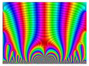
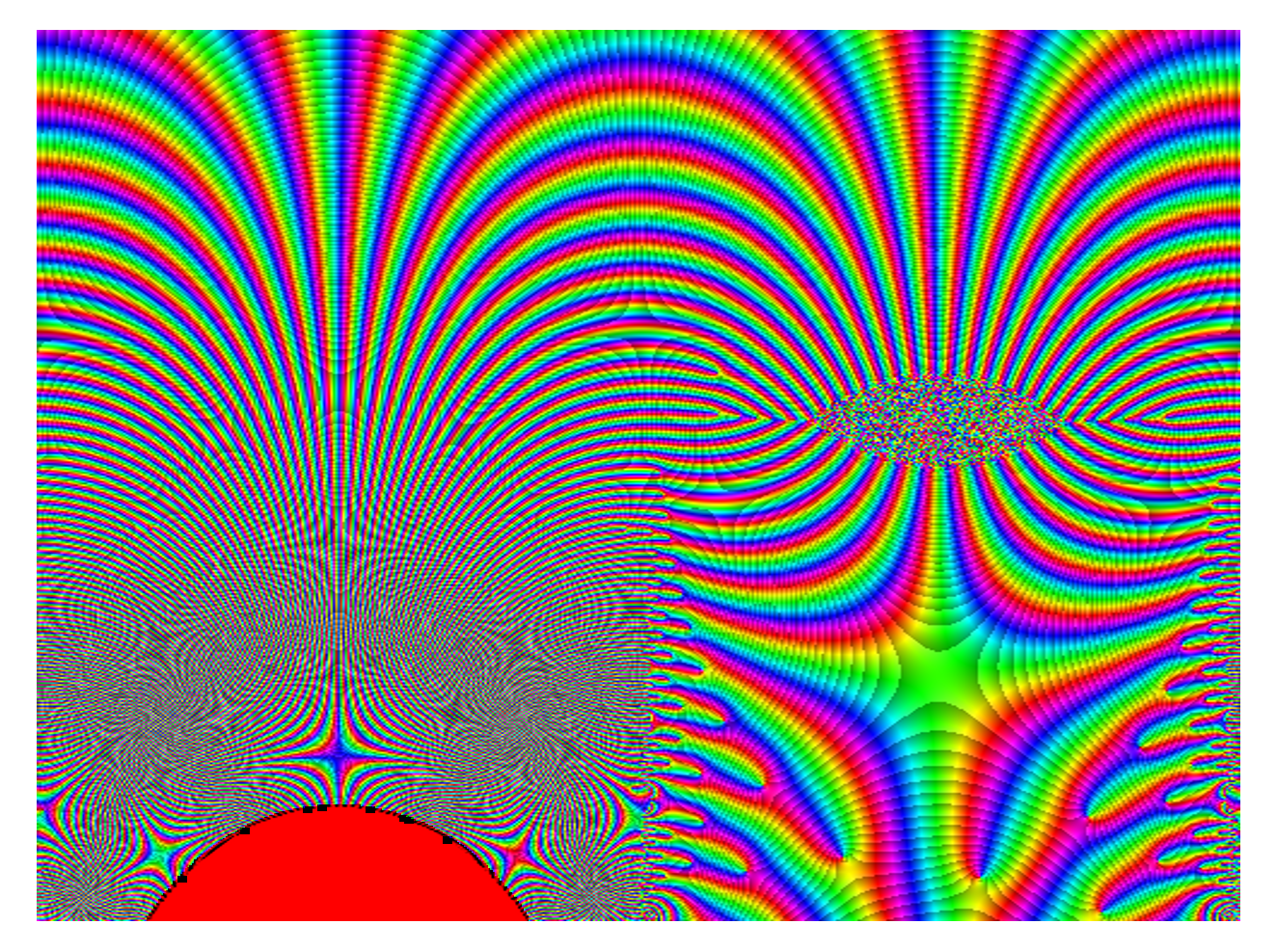
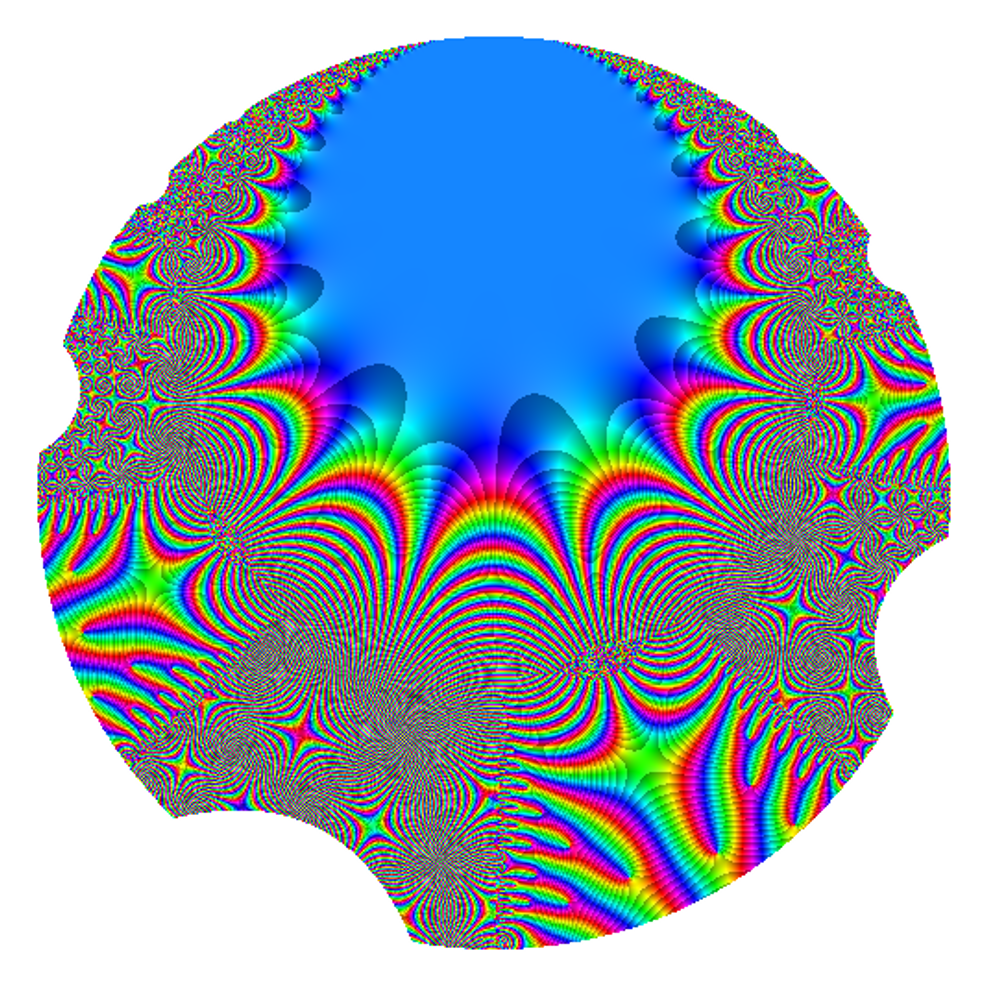
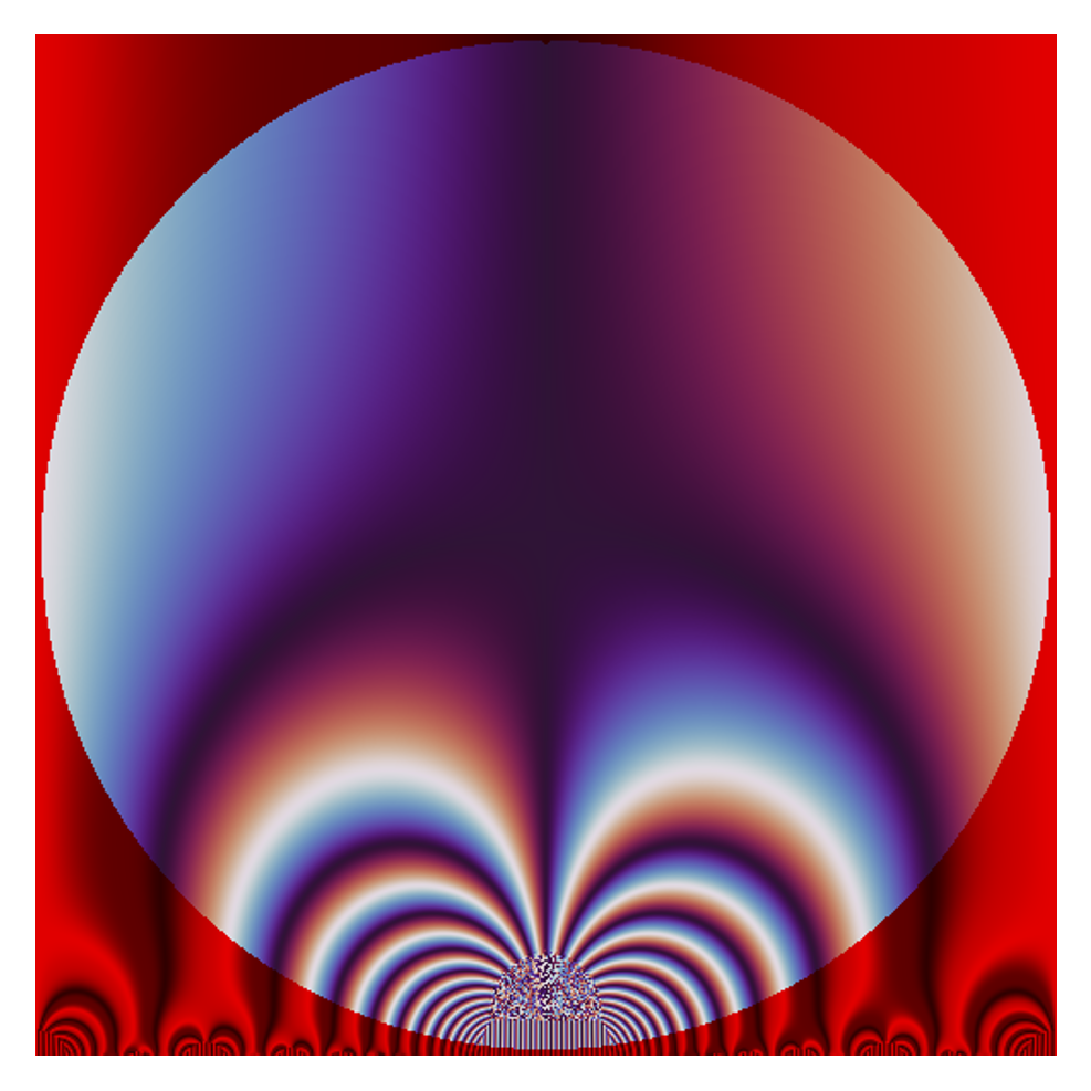
As a final note, I’ll add that I mistyped several times in the preparation of the images for this talk. Included below are a few of the interesting-looking mistakes. The first two resulted from incorrectly applied conformal mappings, while the third came from incorrectly applied color correction.
Info on how to comment
To make a comment, please send an email using the button below. Your email address won't be shared (unless you include it in the body of your comment). If you don't want your real name to be used next to your comment, please specify the name you would like to use. If you want your name to link to a particular url, include that as well.
bold, italics, and plain text are allowed in comments. A reasonable subset of markdown is supported, including lists, links, and fenced code blocks. In addition, math can be formatted using
$(inline math)$or$$(your display equation)$$.Please use plaintext email when commenting. See Plaintext Email and Comments on this site for more. Note also that comments are expected to be open, considerate, and respectful.