mixedmath

The US House of Representatives has 435 voting members (and 6 non-voting members: one each from Washington DC, Puerto Rico, American Samoa, Guam, the Northern Mariana Islands, and the US Virgin Islands). Roughly speaking, the higher the population of a state is, the more representatives it should have.

But what does this really mean?

If we looked at the US Constitution to make this clear, we would find little help. The third clause of Article I, Section II of the Constitution says

Representatives and direct Taxes shall be apportioned among the several States which may be included within this Union, according to their respective Numbers ... The number of Representatives shall not exceed one for every thirty thousand, but each state shall have at least one Representative.

This doesn't give clarity.^{1 1}I omit that in fact it says that the "respective Number" shall be determined by adding to the whole Number of free Persons, including those bound to Service for a Term of Years, and excluding Indians not taxed, three fifths of all other Persons. This was amended by the Fourteenth Amendment. In fact, uncertainty surrounding proper apportionment of representatives led to the first presidential veto.

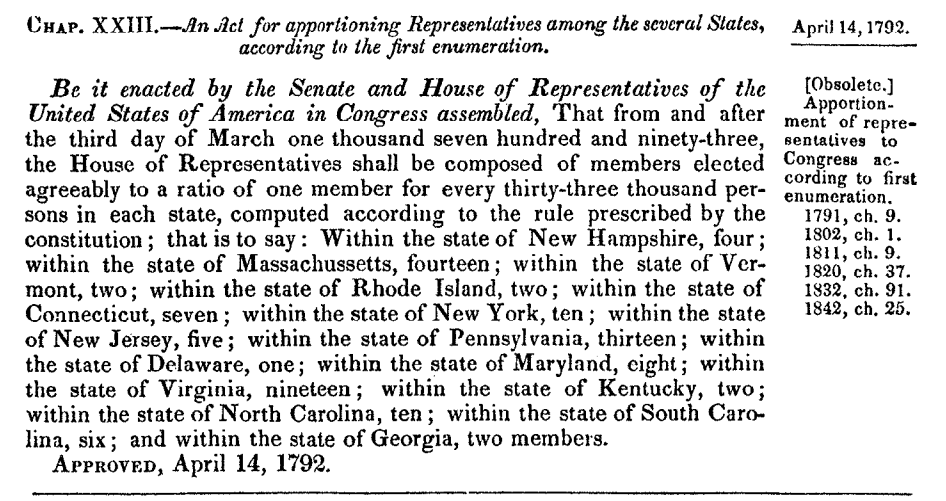
The Apportionment Act of 1792

According to the 1790 Census, there were 3199415 free people and 694280 slaves in the United States.^{2 2}As an aside, I did not know that 1 in every 6 people in the US was a slave at the time. I don't know what to make of this fact, other than that it's remarkably high.

When Congress sat to decide on apportionment in 1792, they initially computed the total (weighted) population of the United States to be 3199415 + (3/5)⋅694280 ≈ 3615923. They noted that the Constitution says there should be no more than 1 representative for every 30000, so they divided the total population by 30000 and rounded down, getting 3615983/30000 ≈ 120.5.

Thus there were to be 120 representatives. If one takes each state and divides their populations by 30000, one sees that the states should get the following numbers of representatives^{3 3}In a later note, I will share my data and code I used to compute the statistics in this note.

State          ideal    rounded_down
Vermont        2.851    2
NewHampshire   4.727    4
Maine          3.218    3
Massachusetts  12.62    12
RhodeIsland    2.281    2
Connecticut    7.894    7
NewYork        11.05    11
NewJersey      5.985    5
Pennsylvania   14.42    14
Delaware       1.851    1
Maryland       9.283    9
Virginia       21.01    21
Kentucky       2.290    2
NorthCarolina  11.78    11
SouthCarolina  6.874    6
Georgia        2.361    2

But here is a problem: the total number of rounded down representatives is only 112. So there are 8 more representatives to give out. How did they decide which to assign these representatives to? They chose the 8 states with the largest fractional "ideal" parts:

1. New Jersey (0.985)
2. Connecticut (0.894)
3. South Carolina (0.874)
4. Vermont (0.851)
5. Delaware (0.851)
6. Massachusetts+Maine (0.838)
7. North Carolina (0.78)
8. New Hampshire (0.727)

(Maine was part of Massachuestts at the time, which is why I combine their fractional parts). Thus the original proposed apportionment gave each of these states one additional representative. Is this a reasonable conclusion?

Perhaps. But these 8 states each ended up having more than 1 representative for each 30000. Was this limit in the Constitution meant country-wide (so that 120 across the country is a fine number) or state-by-state (so that, for instance, Delaware, which had 59000 total population, should not be allowed to have more than 1 representative)?

There is the other problem that New Jersey, Connecticut, Vermont, New Hampshire, and Massachusetts were undoubtedly Northern states. Thus Southern representatives asked, Is it not unfair that the fractional apportionment favours the North?^{4 4}There is a further point of contention. Much of the Southern population (approximately one third) consisted of slaves. The weighting agreed on in the Constitution counted against the Southern states' representative count — or so these states claimed.

Regardless of the exact reasoning, the Secretary of State Thomas Jefferson and Attorney General Edmond Randalph (both from Virginia) urged President Washington to veto the bill, and he did. This was the first use of the Presidential veto.

Afterwards, Congress got together and decided on starting with 33000 people per representative and ignoring fractional parts entirely. The exact method became known as the Jefferson Method of Apportionment, and was used in the US until 1830. The subtle part of the method involves deciding on the number 33000. In the US, the exact number of representatives sometimes changed from election to election. This number is closely related to the population-per-representative, but these were often chosen through political maneuvering as opposed to exact decision.

As an aside, it's interesting to note that this method of apportionment is widely used in the rest of the world, even though it was abandoned in the US.^{5 5}And it is essentially equivalent to the D'Hondt method, proposed by Belgian mathematician D'Hondt in 1878. The presentations of the method are different — D'Hondt's method is presented as an algorithm. We'll return to this later in this note. In fact, it is still used in Albania, Angola, Argentina, Armenia, Aruba, Austria, Belgium, Bolivia, Brazil, Bulgaria, Burundi, Cambodia, Cape Verde, Chile, Colombia, Croatia, the Czech Republic, Denmark, the Dominican Republic, East Timor, Ecuador, El Salvador, Estonia, Fiji, Finland, Guatemala, Hungary, Iceland, Israel, Japan, Kosovo, Luxembourg, Macedonia, Moldova, Monaco, Montenegro, Mozambique, Netherlands, Nicaragua, Northern Ireland, Paraguay, Peru, Poland, Portugal, Romania, San Marino, Scotland, Serbia, Slovenia, Spain, Switzerland, Turkey, Uruguay, Venezuela and Wales — as well as in many countries for election to the European Parliament.

Measuring the fairness of an apportionment method

At the core of different ideas for apportionment is fairness. How can we decide if an apportionment fair?

We'll consider this question in the context of the post-1911 United States — after the number of seats in the House of Representatives was established. This number was set at 433, but with the proviso that anticipated new states Arizona and New Mexico would each come with an additional seat.^{6 6}Actually, in 1959, both Alaska and Hawaii were temporarily given one House seat as they joined the US. Thus in 1959, the House had 437 members. But in 1960, the total seat count returned to 435. So they weren't totally left out.

So given that there are 435 seats to apportion, how might we decide if an apportionment is fair? Fundamentally, this should relate to the number of people each representative actually represents.

For example, in the 1792 apportionment, the single Delawaran representative was there to represent all 55000 of its population, while each of the two Rhode Island representatives corresponded to 34000 Rhode Islanders. Within the House of Representatives, it was as though the voice of each Delawaran only counted 61 percent as much as the voice of each Rhode Islander^{7 7}Being counted as only 3/5 of a person isn't fair, is it?

The number of people each representative actually represent is at the core of the notion of fairness — but even then, it's not obvious.

Suppose we enumerate the states, so that S_i refers to state i. We'll also denote by P_i the population of state i, and we'll let R_i denote the number of representatives allotted to state i.

In the ideal scenario, every representative would represent the exact same number of people. That is, we would have $$\text{pop. per rep. in state i} = \frac{P_i}{R_i} = \frac{P_j}{R_j} = \text{pop. per rep. in state j}$$ for every pair of states i and j. But this won't ever happen in practice.

Generally, we should expect $\frac{P_i}{R_i} \neq \frac{P_j}{R_j}$ for every pair of distinct states. If $$ \frac{P_i}{R_i} > \frac{P_j}{R_j}, \tag{1} $$ then we can say that each representative in state i represents more people, and thus those people have a diluted vote.

Amounts of Inequality

There are lots of pairs of states. How do we actually measure these inequalities? This would make an excellent question in a statistics class (illustrating how one can answer the same question in different, equally reasonable ways) or even a civics class.

A few natural ideas emerge:

• We might try to minimize the differences of constituency size: $\left \lvert \frac{P_i}{R_i} - \frac{P_j}{R_j} \right \rvert$.
• We might try to minimize the differences in per capita representation: $\left \lvert \frac{R_i}{P_i} - \frac{R_j}{P_j} \right \rvert$.
• We might take overall size into account, and try to minimize both the relative constituency size and relative difference in per capita representation.

This last one needs a bit of explanation. Define the relative difference between two numbers x and y to be $$ \frac{\lvert x - y \rvert}{\min(x, y)}. $$

Suppose that for a pair of states, we have that $(1)$ holds, i.e. that representatives in state j have smaller constituencies than in state i (and therefore people in state j have more powerful votes). Then the relative difference in constituency size is $$ \frac{P_i/R_i - P_j/R_j}{P_j/R_j} = \frac{P_i/R_i}{P_j/R_j} - 1. $$ The relative difference in per capita representation is $$ \frac{R_j/P_j - R_i/P_i}{R_i/P_i} = \frac{R_j/P_j}{R_i/P_i} - 1 = \frac{P_i/R_i}{P_j/R_j} - 1. $$ Thus these are the same! By accounting for differences in size by taking relative proportions, we see that minimizing relative difference in constituency size and minimizing relative difference in per capita representation are actually the same.

All three of these measures seem reasonable at first inspection. Unfortunately, they all give different apportionments (and all are different from Jefferson's scheme — though to be fair, Jefferson's scheme doesn't seek to minimize inequality and there is no reason to think it should behave the same).

Each of these ideas leads to a different apportionment scheme, and in fact each has a name.

• Minimizing differences in constituency size is the Dean method.
• Minimizing differences in per capita representation is the Webster method.
• Minimizing relative differences between both constituency size and per capita representation is the Hill (or sometimes Huntington-Hill) method.

Further, each of these schemes has been used at some time in US history. Webster's method was used immediately after the 1840 census, but for the 1850 census the original Alexander Hamilton scheme (the scheme vetoed by Washington in 1792) was used. In fact, the Apportionment Act of 1850 set the Hamilton method as the primary method, and this was nominally used until 1900.^{8 8}There is an anomaly in 1870 that we return to at the very end of this note. The Webster method was used again immediately after the 1910 census. Due to claims of incomplete and inaccurate census counts, no apportionment occurred based on the 1920 census.^{9 9}Non-coincidentally, the size of the House was fixed in 1913 at 435, so the political games leading to slightly larger House sizes every apportionment could not occur. Further, there was large-scale immigration and concentration within urban cities between 1910 and 1920. If one used the census results, then many representatives (especially Republican representatives in what was a newly elected Republican government) would have simply had their seats disappear. So they refused to reapportion.

In 1929 an automatic apportionment act was passed.^{10 10}Largely thanks to the efforts of Republican Senator Arthur Vandenberg of Michigan, who repeatedly addressed the nation by radio on the necessity of reapportionment based on the census. He also helped set up the UN and was a major voice in the Republican Party who helped guide the party away from isolationism to internationalism. He was the chair of the Senate Foreign Relations Committee from 1947–1949, during which he supported (Democratic) President Truman's Cold War policies, the Truman Doctrine, the Marshall Plan, and NATO. In it, up to three different apportionment schemes would be provided to Congress after each census, based on a total of 435 seats:

1. The apportionment that would come from whatever scheme was most recently used. (In 1930, this would be the Webster method).
2. The apportionment that would come from the Webster method.
3. The apportionment that would come from the newly introduced Hill method.

If one reads congressional discussion from the time, then it will be good to note that Webster's method is sometimes called the method of major fractions and Hill's method is sometimes called the method of equal proportions. Further, in a letter written by Bliss, Brown, Eisenhart, and Pearl of the National Academy of Sciences, Hill's method was declared to be the recommendation of the Academy.^{11 11}Report to the President of the National Academy, 1929. This can be read in the collections of reports of the National Academy of Sciences. From 1930 on, Hill's method has been used.

Why use the Hill method?

The Hamilton method led to a few paradoxes and highly counterintuitive behavior that many representatives found disagreeable. In 1880, a paradox now called the Alabama paradox was noted. When deciding on the number of representatives that should be in the House, it was noted that if the House had 299 members, Alabama would have 8 representatives. But if the House had 300 members, Alabama would have 7 representatives — that is, making one more seat available led to Alabama receiving one fewer seat.

The problem is the fluctuating relationships between the many fractional parts of the ideal number of representatives per state (similar to those tallied in the table in the section The Apportionment Act of 1792).

Another paradox was discovered in 1900, known as the Population paradox. This is a scenario in which a state with a large population and rapid growth can lose a seat to a state with a small population and smaller population growth. In 1900, Virginia lost a seat to Maine, even though Virginia's population was larger and growing much more rapidly.

In particular, in 1900, Virginia had 1854184 people and Maine had 694466 people, so Virginia had 2.67 times the population as Maine. In 1901, Virginia had 1873951 people and Maine had 699114 people, so Virginia had 2.68 times the number of people. And yet Hamilton apportionment would have given 10 seats to Virginia and 3 to Maine in 1900, but 9 to Virginia and 4 to Maine in 1901.

Central to this paradox is that even though Virginia was growing faster than Maine the rest of the nation was growing fast still, and proportionally Virginia lost more because it was a larger state. But it's still paradoxical for a state to lose a representative to a second state that is both smaller in population and is growing less rapidly each census.^{12 12}This analysis was taken from Balinski and Young, Fair representation: meeting the ideal of one man, one vote.

The Hill method can be shown to not suffer from either the Alabama paradox or the Population paradox. That it doesn't suffer from these paradoxical behaviours and that it seeks to minimize a meaningful measure of inequality led to its adoption in the US.^{13 13}But it isn't perfect! Balinski and Young (the same two mathematicians from the previous footnote) also proved that there doesn't exist an apportionment system that both gives results very near the ideal results and which is immune to both the Alabama paradox and the population paradox. Hard choices must be made

Understanding the modern Hill method in practice

Since 1930, the US has used the Hill method to apportion seats for the House of Representatives. But as described above, it may be hard to understand how to actually apply the Hill method. Recall that P_i is the population of state i, and R_i is the number of representatives allocated to state i. The Hill method seeks to minimize $$ \frac{P_i/R_i - P_j/R_j}{P_j/R_j} = \frac{P_i/R_i}{P_j/R_j} - 1 $$ whenever P_i/R_i > P_j/R_j. Stated differently, the Hill method seeks to guarantee the smallest relative differences in constituency size.

We can work out a different way of understanding this apportionment that is easier to implement in practice.

Suppose that we have allocated all of the representatives to each state and state j has R_j representatives, and suppose that this allocation successfully minimizes relative differences in constituency size. Take two different states i and j with P_i/R_i > P_j/R_j. (If this isn't possible then the allocation is perfect).

We can ask if it would be a good idea to move one representative from state j to state i, since state j's constituency sizes are smaller. This can be thought of as working with R_i′=R_i + 1 and R_j′=R_j − 1. If this transfer lessens the inequality then it should be made — but since we are supposing that the allocation successfully minimizes relative difference in constituency size, we must have that the inequality is at least as large. This necessarily means that P_j/R_j′>P_i/R_i′ (since otherwise the relative difference is strictly smaller) and $$ \frac{P_jR_i'}{P_iR_j'} - 1 \geq \frac{P_iR_j}{P_jR_i} - 1 $$ (since the relative difference must be at least as large). This is equivalent to $$ \frac{P_j(R_i+1)}{P_i(R_j-1)} \geq \frac{P_iR_j}{P_jR_i} \iff \frac{P_j^2}{(R_j-1)R_j} \geq \frac{P_i^2}{R_i(R_i+1)}. $$ As every variable is positive, we can rewrite this as $$ \frac{P_j}{\sqrt{(R_j - 1)R_j}} \geq \frac{P_i}{\sqrt{R_i(R_i+1)}}. \tag{2} $$

We've shown that $(2)$ must hold whenever P_i/R_i > P_j/R_j in a system that minimizes relative difference in constituency size. But in fact it must hold for all pairs of states i and j.

Clearly it holds if i = j as the denominator on the left is strictly smaller.

If we are in the case when P_j/R_j > P_i/R_i, then we necessarily have the chain P_j/(R_j − 1)>P_j/R_j > P_i/R_i > P_i/(R_i + 1). Multiplying the inner and outer inequalities shows that $(2)$ holds trivially in this case.

This inequality shows that the greatest obstruction to being perfectly apportioned as per Hill's method is the largest fraction $$ \frac{R_i}{\sqrt{P_i(P_i+1)}} $$ being too large. (Some call this term the Hill rank-index).

An iterative Hill apportionment

This observation leads to the following iterative construction of a Hill apportionment. Initially, assign every state 1 representative (since by the Constitution, each state gets at least one representative). Then, given an apportionment for n seats, we can get an apportionment for n + 1 seats by assigning the additional seat the any state i which maximizes the Hill rank-index $R_i/\sqrt{P_i(P_i+1)}$.

Further, it can be shown that there is a unique apportionment in Hill's method (except for ties in the Hill rank-index, which are exceedingly rare in practice). Thus the apportionment is unique.

This is very quickly and easily implemented in code. In a later note, I will share the code I used to compute the various data for this note, as well as an implementation of Hill apportionment.

Additional notes: Consequences of the 1870 and 1990 Apportionments

The 1870 Apportionment

Officially, Dean's method of apportionment has never been used. But it was perhaps used in 1870 without being described. Officially, Hamilton's method was in place and the size of the House was agreed to be 292. But the actual apportionment that occurred agreed with Dean's method, not Hamilton's method. Specifically, New York and Illinois were each given one fewer seat than Hamilton's method would have given, while New Hampshire and Florida were given one additional seat each.

There are many circumstances surrounding the 1870 census and apportionment that make this a particularly convoluted time. Firstly, the US had just experienced its Civil War, where millions of people died and millions others moved or were displaced. Animosity and reconstruction were both in full swing. Secondly, the US passed the 14th amendment in 1868, so that suddenly the populations of Southern states grew as former slaves were finally allowed to be counted fully.

One might think that having two pairs of states swap a representative would be mostly inconsequential. But this difference — using Dean's method instead of the agreed on Hamilton method, changed the result of the 1876 Presidential election. In this election, Samuel Tilden won New York while Rutherford B. Hayes won Illinois, New Hampshire, and Florida. As a result, Tilden received one fewer electoral vote and Hayes received one additional electoral vote — and the total electoral voting in the end had Hayes win with 185 votes to Tilden's 184.

There is still one further mitigating factor, however, that causes this to be yet more convoluted. The 1876 election is perhaps the most disputed presidential election. In Florida, Louisiana, and South Carolina, each party reported that its candidate had won the state. Legitimacy was in question, and it's widely believed that a deal was struck between the Democratic and Republican parties (see wikipedia and 270 to win). As a result of this deal, the Republican candidate Rutherford B. Hayes would gain all disputed votes and remove federal troops (which had been propping up reconstructive efforts) from the South. This marked the end of the "Reconstruction" period, and allowed the rise of the Democratic Redeemers (and their rampant black voter disenfranchisement) in the South.

The 1990 Apportionment

Similar in consequence though not in controversy, the apportionment of 1990 influenced the results of the 2000 presidential election between George W. Bush and Al Gore (as the 2000 census is not complete before the election takes place, so the election occurs with the 1990 electoral college sizes). The modern Hill apportionment method was used, as it has been since 1930. But interestingly, if the originally proposed Hamilton method of 1792 was used, the electoral college would have been tied at 269^{14 14}Note there was one Gore abstention in 2000 . If Jefferson's method had been used, then Gore would have won with 271 votes to Bush's 266.

These decisions have far-reaching consequences!

Sources

1. Balinski, Michel L., and H. Peyton Young. Fair representation: meeting the ideal of one man, one vote. Brookings Institution Press, 2010.
2. Balinski, Michel L., and H. Peyton Young. "The quota method of apportionment." The American Mathematical Monthly 82.7 (1975): 701-730.
3. Bliss, G. A., Brown, E. W., Eisenhart, L. P., & Pearl, R. (1929). Report to the President of the National Academy of Sciences. February, 9, 1015-1047.
4. Crocker, R. House of Representatives Apportionment Formula: An Analysis of Proposals for Change and Their Impact on States. DIANE Publishing, 2011.
5. Huntington, The Apportionment of Representatives in Congress, Transactions of the American Mathematical Society 30 (1928), 85–110.
6. Peskin, Allan. "Was there a Compromise of 1877." The Journal of American History 60.1 (1973): 63-75.
7. US Census Results
8. US Constitution
9. US Congressional Record, as collected at https://memory.loc.gov/ammem/amlaw/lwaclink.html
10. George Washington's collected papers, as archived at https://web.archive.org/web/20090124222206/http://gwpapers.virginia.edu/documents/presidential/veto.html
11. Wikipedia on the Compromise of 1877, at https://en.wikipedia.org/wiki/Compromise_of_1877
12. Wikipedia on Arthur Vandenberg, at https://en.wikipedia.org/wiki/Arthur_Vandenberg

Leave a comment

Comment via email